Welcome to the Photometric Redshift (PZ) Data Challenge
The Dark Energy Science Collaboration (DESC) invites researchers, data scientists, and astronomers to participate in the Photometric Redshift (PZ) Data Challenge, a collaborative effort to advance methods for estimating the distances to distant galaxies. Photometric redshifts, derived from multi-band brightness measurements, are essential for cosmological surveys like the Legacy Survey of Space and Time (LSST), enabling us to map the universe’s structure and probe the nature of dark energy. This challenge provides a unique opportunity to test and benchmark algorithms on realistic simulated data, compare approaches across diverse methodologies—from template fitting to machine learning—and help shape the tools that will unlock discoveries from next-generation sky surveys.
The challenge is framed as a series of sets of PZ estimations tasks using increasingly realistic data.
Set up the pz_data_challenge package and download challenge data
Information about the input data
How to submit an entry to the challenge
Description of challenge tasks
Background Information
Introduction
Redshift inference is a key element of many DESC science goals, and redshift uncertainty is one of the leading contributors to overall uncertainty on cosmological models from imaging survey data. Precursor surveys took a variety of approaches to this problem, accounting for differences in underlying data as well as modeling approaches. In all cases, redshift uncertainty was significantly larger than the DESC Science Requirements listed in the LSST DESC Science Requirements Document.
This state of the art motivates a data challenge to characterize and improve existing methods, as well as to provide infrastructure for the development of improved methods. Overall, this requires generating uniform input catalogs to use and infrastructure for comparing output redshift posteriors to each other and to simulated truth catalogs.
Photometric redshift basics
Photometric redshift estimation involves taking a catalog of galaxies for which we have observations in several different filters and have measured the brightness of the galaxies in those bands, and using that information to estimate the redshift of the galaxies. For LSST we expect to have measurements in 6 bands: ’u’, ’g’, ’r’, ’i’, ’z’, and ’y’, covering a wavelength range from approximately 320 to 1600 nanometers. For the Roman space telescope, this will extend from about 500 to 2300 nanometers.
Much of the information used to estimate photometric redshifts derives from the ’Balmer break’ present in the rest frame of many spectra at 400 nm. As the break crosses into different optical filters with increasing redshift, the differences in magnitudes between filters carry information about the redshift;
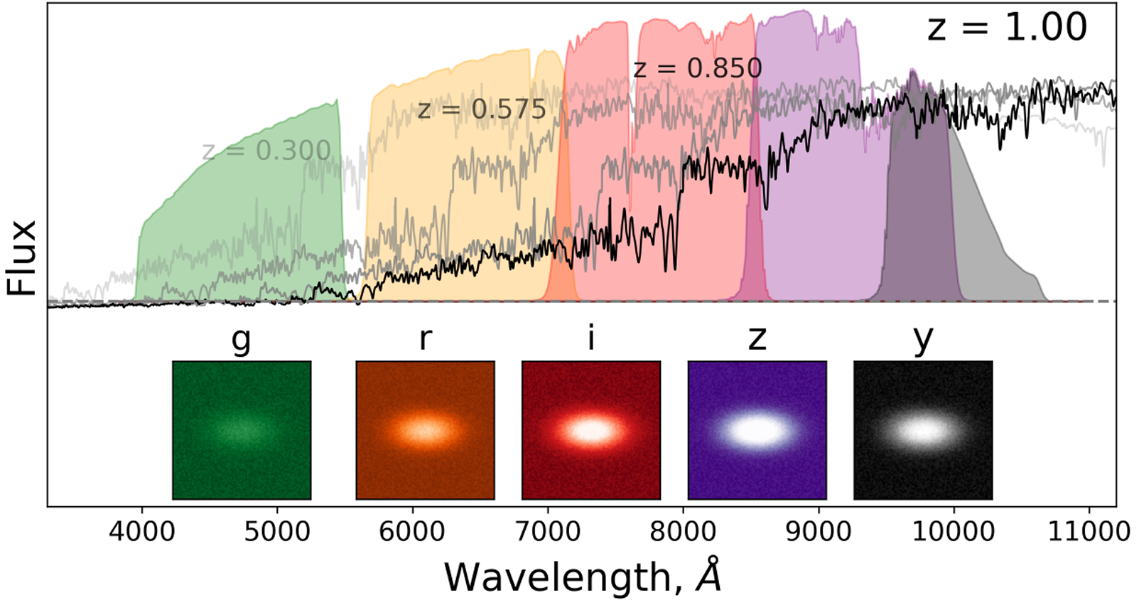
Fig. 1 A passive galaxy at different redshifts and how it will show up in various optical filters, giving us the ability to estimate its redshift and therefore distance. For many galaxies, the so-called ‘Balmer break’ at 400 nm is a reliable feature that causes the flux to drop severely in bluer filters. Figure and caption by Jamie McCullough.
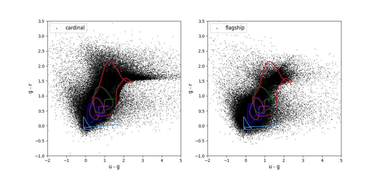
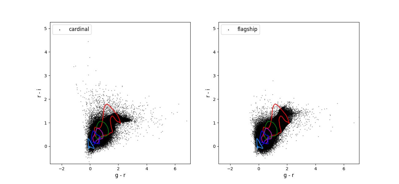
This can also be seen when plotting redshifts as a function of derived colors, i.e., differences in magnitudes between filters;
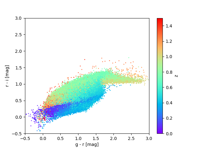
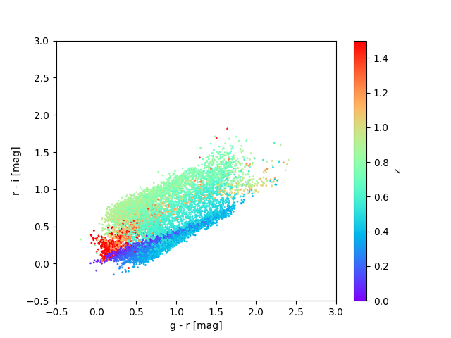
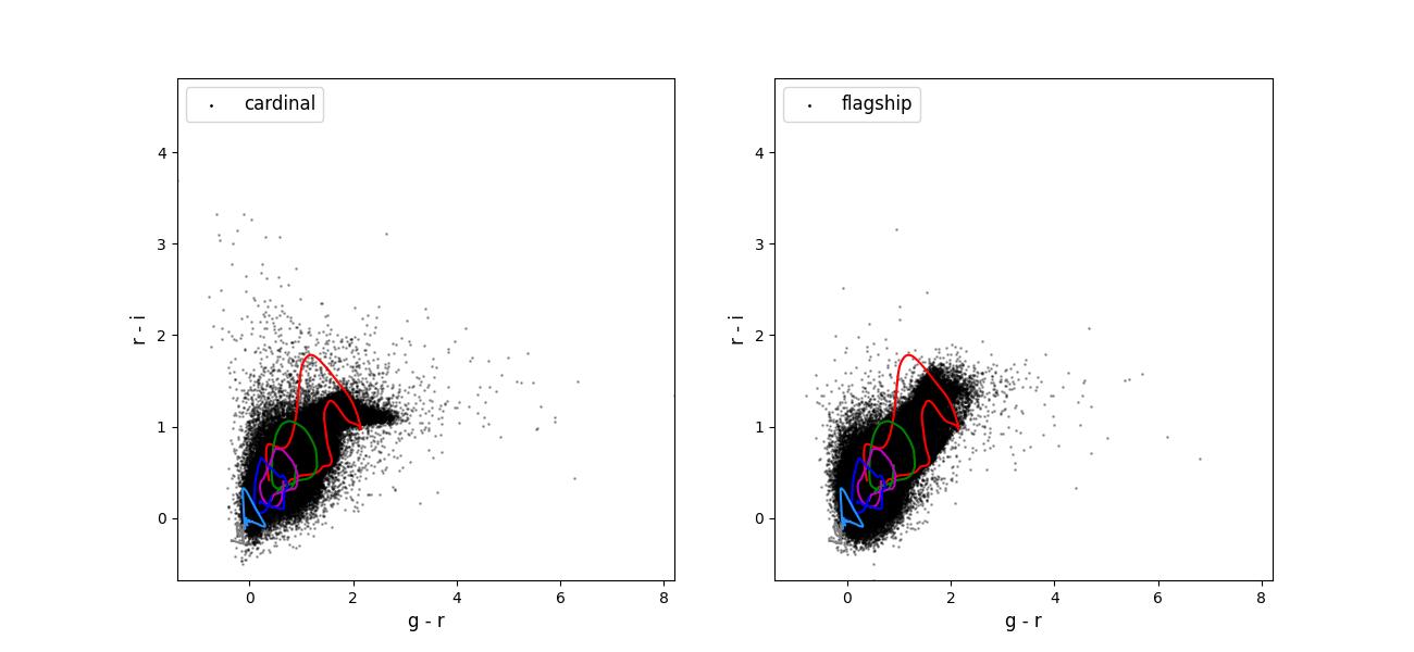
Redshifts plotted as a function of r-i versus g-r colors for a sample of objects in the cardinal (left) and flagship (right) simulations. These are plotted for the data for task set 1, i.e., for a sample of objects with i < 23.
This overly simple picture is complicated somewhat by the fact that different galaxies have different intrinsic spectra and colors:
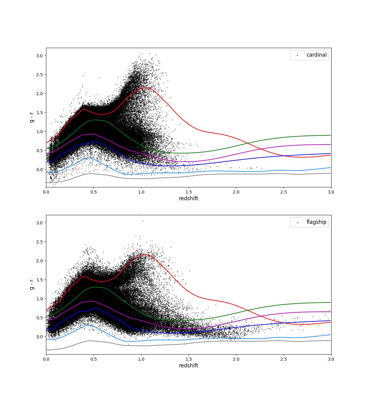
Fig. 2 Color (g-r) plotted as a function of redshift for a sample of objects in the cardinal (top) and flagship (bottom) simulations. These are plotted for the data for task set 1, i.e., for a sample of objects with i < 23. The overlaid lines show the templates for several different types of galaxies.
This is further complicated by the fact that reference redshifts, typically obtained by spectroscopy, slitless spectroscopy (i.e., GRISM measurements), or narrowband photometric measurements, are not a representative sample, as they are much easier to obtain for brighter objects. Depending on the method used to obtain the reference redshifts, they are also susceptible to errors such as confusing different spectral lines or confusion of blended objects. Some of the tasks in this data challenge encourage participants to try to address these complications.
Information about the PZ Data Challenge
Challenge Format
The PZ data challenge comprises a series of sets of tasks for participants. Submissions will be evaluated to determine how ready various algorithms are to be used for cutting-edge analysis based on how well they perform on the various tasks. Readiness will be evaluated on a few different fronts: 1) Does the algorithm meet performance requirements? 2) Is it robust, flexible, and relatively easy to use on different datasets? 3) Is it scalable up to the scales we will need to use it at?
This document and the associated web pages describe the data being provided to participants, the tasks they will be asked to perform, the expected format for submission and the metrics by which the algorithm readiness will be evaluated.
Scope and Timeline
The data challenge will include two major parts, with a set of tasks emulating increasingly realistic scenarios in each part. The first part, \(p(z)\) estimation, will focus on estimating the redshift of individual objects. The second part, tomography and \(n(z)\) estimation, will focus on assigning objects to tomographic bins and estimating the distribution of redshifts in each bin.
The data challenge will run from April 13, 2026 to September 2026. The first set of data and tasks related to \(p(z)\) estimation will be released on April 13 and will close on July 17, 2026. A second set of data and tasks related to more realistic \(p(z)\) estimation scenarios and \(n(z)\) estimation will be released on June 1 and will close in September 2026..
Preliminary results will be released in August 2026, with a technical note summarizing those results to follow shortly thereafter and a comprehensive journal publication to follow later.
Installing and setting up the pz_data_challenge package
The pz_data_challenge package will provide participants with tools
to access data, set up submissions, estimate performance metrics and
format submissions. This can be set up with a few small variants on the
standard GitHub package setup procedure. Before starting you should
pick a name for your submission, e.g., “example”.
# Create a conda environment
conda create --name pzdc python=3.13

# Clone the pz_data_challenge repository (or your fork of the repository)
git clone git@github.com:LSSTDESC/pz_data_challenge.git
# or git clone https://github.com/LSSTDESC/pz_data_challenge.git

# Go into the directory
cd pz_data_challenge

# Install the code in "editable" mode
pip install -e ".[dev]"

# Use the provided script to set up your submission.
# Here you should provide the name of your submission
python scripts/prepare_submission.py <submission_name>
This final step will copy the input data files to
pz_data_challenge/public, and set up the three files you will need
to submit your entry.
The notebooks in the pz_data_challenge/nb area give examples of how
to access the data and create some of the diagnostic plots that were
used to validate the data.
Submission mechanism
Submission will take the form of pull request in the
pz_data_challenge repository. Detailed instructions on how to submit
an entry are provided in Sec. 5 of this
document.
Challenge Input Data
The preparation of the challenge data is described in the appendices.
The data are available as a tar archive that is downloaded and
unpacked as part of the pz_data_challenge setup procedure.
Each task set in the data challenge has an associated set of files. Typically these will be a collection of training files that contain photometric data and reference redshifts, and a second set of files that contain photometric data but do not include redshifts. Each task set will involve estimating something about the redshifts or redshift distributions in the test files.
Typically there will be several training and test files for a particular task set, covering different scenarios and using different input simulations.
Input data format
The input data for the challenge are presented in HDF5 files. The naming
convention for the files is
{challenge}_{taskset}_{simulation}_{label}_{scenario}.hdf5. The
meanings of the various fields are:
Field |
Description |
|---|---|
challenge |
Challenge associated with file |
taskset |
Task set associated with file |
simulation |
Simulation used to produce file (“cardinal” or “flagship”) |
label |
File label (e.g., “test”, “training”) |
scenario |
Data scenario (e.g., “1yr”, “10yr”) |
The columns in the files are:
Column |
Description |
|---|---|
redshift |
True redshift (training files only) |
ra |
Right ascension (training files only) |
dec |
Declination (training files only) |
object_id |
Unique object ID |
mag_{band}_lsst |
Magnitude in LSST {band} |
mag_{band}_lsst_err |
Magnitude uncertainty in LSST {band} |
mag_{band}_roman |
Magnitude in Roman {band} |
mag_{band}_roman_err |
Magnitude uncertainty in Roman {band} |
We note that we use np.nan to in the magnitude columns to signify non-detections.
We note that the table-io package installed with
pz_data_challenge provides a command line interface
to convert files from hdf5 format to other formats such as
parquet tables or pandas data frames.
# convert a hdf5 file to pandas dataframe in a parquet file
tables-io convert
  --input public/pz_challenge_taskset_1_cardinal_test_10yr.hdf5
  --output public/pz_challenge_taskset_1_cardinal_test_10yr.pq
Challenge Submissions
Challenge subtask types
The challenge is organized as a series of sets of tasks using increasingly realistic representations of the data. In general, each set of tasks includes 3 subtasks.
Estimate either per-object \(p(z)\) or ensemble \(n(z)\) distributions for a set of different scenarios and provide the estimates in a specified format.
Provide trained models for the different scenarios and a Python function that can be used to generate the estimates from subtask 1 on an arbitrary dataset.
Provide a Python function that can be used to generate the models and estimates from subtasks 1 and 2 on arbitrary datasets.
The \(p(z)\) estimates in subtask 1 and the trained models in
subtask 2 should be provided in a compressed tar file, which are
described below. Templates and instructions for the Python functions
needed for subtasks 2 and 3 will be provided and are described below.
Data format for per-object \(p(z)\) estimates
The \(p(z)\) estimates should be submitted in qp format, which
allows users to specify a complete \(p(z)\) distribution for each
object, as well as summary statistics for each object.
The qp package supports several different representations of
\(p(z)\), such as different functional forms as well as interpolated
grids, histograms, and others.
For users unfamiliar with qp, we highly recommend representing the
\(p(z)\) as either an interpolated grid or a Gaussian mixture model.
# Interpolated grid
import qp
import numpy as np
# Define the x-grid. Note that we put all the
# p(z) on the same x-grid
xvals = np.array([0,0.5,1,1.5,2])
# Define the y-values. Note we provide n_grid_points x n_objects
# values, as we need to provide a y-value at each grid point
# for each object.
yvals = np.array(
 [
   [0.01,0.2,0.3,0.2,0.01],
   [0.1,0.3,0.5,0.2,0.05]
 ]
)
ensemble = qp.interp.create_ensemble(xvals,yvals)
ensemble.write_to(<output_filename.hdf5>)
# Mixture model
import qp
import numpy as np
# Define the means, standard deviations, and weights.
# These should each have shape n_objects, n_components.
# In this case we are defining 3 objects with 2-Gaussian
# representations.
# For each object the weights should sum to 1, or they
# will be normalized.
means = [[0.3, 0.4], [0.5, 0.5], [0.6, 0.8]]
stds = [[0.2, 0.4], [0.1, 0.3], [0.05, 0.3]]
weights = [[0.8, 0.2], [0.7, 0.3], [0.8, 0.2]]
ens = qp.mixmod.create_ensemble(means=means,stds=stds,weights=weights)
ensemble.write_to(<output_filename.hdf5>)
The submission files should use the same file name conventions defined
in Tab. 1. The labels will typically be
pz_estimate or pz_model and will be specified in the
descriptions of the various tasks, e.g.,
pz_challenge_taskset_1_cardinal_pz_estimate_1yr.hdf5 or
pz_challenge_taskset_1_cardinal_pz_model_1yr.pkl.
All of these files should then be joined into a tar file, which
should then be placed somewhere it can be download. The URL for the
tar should be specified in tests/test_{submission}.py
SUBMISSION_NAME = "example"
SUBMISSION_URL = "https://your.institution.edu/submit_example.tgz"
Format for estimation-only Python functions and trained models
For the second subtask, submissions should provide trained models and implement a function to run estimation using those trained models on the test files provided for each task set. The function will look something like this:
def run_taskset_1_estimation_only(
    model_file: str | Path,
    test_file: str | Path,
    output_file: str | Path,
) -> None:
    # do stuff and write p(z) estimates to "output_file"
or
def run_taskset_2_estimation_only(
    model_file: str | Path,
    test_file: str | Path,
    output_file: str | Path,
) -> None:
    # do stuff and write p(z) estimates to "output_file"
Templates for these functions are provided in the file
tests/test_{submission}.py created as part of the setup.
Format for training and estimation Python functions
For the third subtask, submissions should implement a function to train models and run estimation using those trained models on the training and test files provided for each task set. The function will look something like this:
def run_taskset_1_training_and_estimation(
    train_file: str | Path,
    test_file: str | Path,
    output_file: str | Path,
) -> None:
    # train a model using the "train_file" and make p(z) estimates
    # and write them to "output_file"
or
def run_taskset_2_training_and_estimation(
    train_file: str | Path,
    test_file: str | Path,
    output_file: str | Path,
) -> None:
    # train a model using the "train_file" and make p(z) estimates
    # and write them to "output_file"
Templates for these functions are provided in the file
tests/test_{submission}.py created as part of the setup.
Submission mechanism details
Submissions will take the form of a pull request on the
pz_data_challenge repository and will include:
A file
tests/test_{submission}.pythat includes the URL from which the compressedtarfile should be downloaded as well as the Python functions for subtasks 2 and 3. When created this will contain empty placeholder functions that will need to be implemented.A file
requirements_{submission}.txtthat should be modified to includepippackage names of any packages that need to be installed in order to run the functions in subtasks 2 and 3.A file
.github/workflows/submit_{submission}.yamlto run the submission validation in a GitHub action. This should not need to be modified unless the prerequisite installation requires more than justpipinstalling packages.
All three of these files are created by the
scripts/prepare_submission.py script.
You will need modify the tests/test_{submission}.py to give the
location of the tar file containing the PZ estimates and trained
models.
See https://github.com/LSSTDESC/pz_data_challenge/pull/6 for an example of a submission.
Submission validation
The wrapping functions provided in the tests/test_{submission}.py
file implement a number of checks on the data. Specifically, for each
expected file they check that:
the file exists;
the file contains a valid
qpensemble;the
qpensemble includes ancillary data;the ancillary data includes a ’zmode’ column with redshift estimates;
the ancillary data includes an ’object_id’ column;
the object_ids in the submission file match the associated test file.
If any of these checks fail, the GitHub action triggered by the submission will fail and report the cause of the failure. Note that the github actions occasionally fail to download the data files. If this happens simply rerunning the action typically succeeds.
The easiest way to test that you have correctly implemented the required functions is simply to run these commands.
# Make sure that you have installed any packages you need
pip install -r requirement_{submission_name}.txt

# Run the functions you have provided as unit tests
py.test tests/test_{submission_name}.py
if this succeeds, you can use a provided script to help you open the pull request for your submission.
# run the submission helper script.
python scripts/submit.py {submission_name}
Note that the help script only prints the required commands, it does not run them. In short the command are:
# Check status of your local git clone by running git status, and make
# sure that you are on the branch submit/{submission_name} and do not
# have any files added or modified
git status

# Add your files to git
git add .github/workflows/submit_example.yaml
  requirements_example.txt
  tests/test_example.py

# Commit your files to your branch:
git commit -m "Submitting {submission_name}"
  .github/workflows/submit_{submission_name}.yaml
  requirements_{submission_name}.txt
  tests/test_{submission_name}.py

# Push your commit
git push --set-upstream origin submit/{submission_name}

# Pushing to git should give you a URL that you can visit to create a
# pull request, for example:
#   https://github.com/LSSTDESC/pz_data_challenge/pull/new/submit/example
# Visit that URL and create a pull request, then add the 'submission'
# label to the PR.
# Finally, make sure that the github action validating your submission
# succeeds and fix any issues.
Submission aids
A few scripts are provided to help you.
scripts/download_public.py: downloads and unpacks the public data.scripts/prepare_submission.py: sets up your area for a submission, creates the needed files from templates and downloads the public data. Suggests that you create a branch for you submission.scripts/remove_submission_files.py: removes the submission files if you need to start over.scripts/run_metrics.py: run perfomance metrics on files in a = submission you have created.py.test tests/test_{submission_name}.py: validates all the parts of your submission, checking that you have created all the required files and that they are properly formatted.
Feedback after submission
Approximately every 2 weeks we will merge the various PRs that are passing the github actions, run performance metrics and update the website with information about their performance.
Metrics and Assessment Criteria
We will use a number of different metrics to assess the performance of the submitted algorithms. Many of these metrics, as well as the motivations behind them, are defined and discussed in [1]
Metrics for per-object point estimates
Performance on per-object point estimates, i.e., providing a single best estimate of the redshift of each object in the test sample. All of our point-estimate metrics first compute the scaled residual, \(\Delta_i\), between the point estimate for each object, \(z_{p,i}\), and the true redshift for that object, \(z_{t,i}\):
We then use this to construct the following metrics; see [1] for more details:
Biasis simply the median of \(\Delta_i\).OutlierRateis the fraction of the \(\Delta\) distribution outside of \([0, {\rm max}(0.06, 3\sigma_{\rm iqr})]\).SigmaMADis an estimate of the standard deviation of the median absolute deviation (MAD), which is computed as\[{\sigma_{\rm MAD}} = 1.4862\,{\rm median}(|\Delta_i - {\rm median}(\Delta)|).\]
Metrics for per-object \(p(z)\) distributions
We will also assess the algorithm’s ability to provide a precise and accurate estimate of the posterior distribution, \(p(z)\), for each object using the following metrics.
Conditional Density Loss (
CDELoss): We implement the method in [2] to compute this metric. A better estimation should return a smaller CDE loss.Probability Integral Transform (PIT): This is the cumulative distribution function of the photo-\(z\) PDF evaluated at the galaxy’s true redshift for each galaxy in the catalog, i.e., \({\rm PIT} = \int_{0}^{z_t} p(z)\, dz\). Following [3], we provide the PIT-QQ (quantile-quantile) diagram, where the PIT distribution is directly compared to the ideal uniform distribution. A diagonal PIT-QQ diagram indicates a good estimation. An example of the PIT-QQ plot is shown below. We will then use three metrics to quantify how well the PIT distribution matches the ideal: the Kolmogorov-Smirnov (KS) test, the Root Mean Square Error (RMSE), and the Kullback-Leibler divergence (KL divergence).
Metrics for computational usability and performance
We will assess relevant aspects of the computational performance that will affect usability and scaling.
Ease of use: We will assess whether the algorithm is easy to install and can be run on the different task sets without needing excessively complicated additional configuration files.
Training time: How quickly the algorithm trains models, and how this scales with the training sample size. Here we mainly want to ensure that the training time will not dominate the iteration cycle. Taking several minutes to train on 100k objects is fine; taking hours to do so would be problematic.
Model size: How large the trained model files are, and how this scales with the training sample size. Again, we mainly want to ensure that the model size will not tax our resources. If the model files are an order of magnitude larger than the input data files, we might worry.
Estimation time: How quickly the algorithm estimates redshifts per object. This will determine the use cases for which we might use the algorithm. We can run an algorithm that takes a few ms per object on all of the billions of galaxies we will have in the final LSST sample; for an algorithm that takes a few seconds per object, we would probably be constrained to only run it on much smaller particular datasets for specific science cases, such as samples of supernovae or strongly lensed objects.
Output data size per object: How large the output files with the \(p(z)\) estimates are. For a
qpinterpolated grid representation with 300 points, these would be about 2.4 kB per object, which is large but manageable, whereas for a Gaussian mixture model with 5 Gaussians, this would be close to 120 bytes per object.
Information about Challenge Data Preparation
Input simulations
The challenge employs simulated galaxy catalogs derived from two complementary N-body cosmological simulations: the Cardinal simulations and the Flagship simulation. These synthetic datasets provide a controlled environment where the true redshifts are known by construction, enabling rigorous validation of photometric redshift algorithms and systematic assessment of their performance characteristics.
The Cardinal simulations comprise a suite of high-resolution N-body simulations specifically designed to explore the sensitivity of cosmological observables to variations in fundamental cosmological parameters. The simulations employ state-of-the-art semi-analytic models to populate dark matter halos with galaxies, incorporating realistic prescriptions for star formation, dust attenuation, and spectral energy distribution modeling.
The Flagship simulation represents a single, ultra-large cosmological simulation run with fiducial cosmological parameters consistent with current observational constraints. With a volume exceeding several cubic gigaparsecs, the Flagship provides statistical power to probe rare objects and the high-mass end of the galaxy population. Its primary purpose in the photometric redshift challenge is to provide a realistic mock catalog that captures the full complexity of galaxy populations across cosmic time, including correlations between galaxy properties, environmental dependencies, and the intricate relationships between spectral features and redshift.
Together, these complementary simulation suites enable challenge participants to test both the accuracy and the robustness of their photometric redshift estimation methods under realistic observational conditions.
Emulating observational effects
To bridge the gap between the idealized simulation outputs and realistic survey observations, we employ the RAIL (Redshift Assessment Infrastructure Layers) software package to emulate observational effects. RAIL provides a modular framework for injecting realistic photometric uncertainties, applying survey-specific selection functions, and simulating the measurement errors characteristic of modern large-scale imaging surveys. This processing ensures that the simulated galaxy catalogs reflect the complexities of actual observations, including magnitude-dependent photometric scatter, incomplete sky coverage, and the effects of source blending in crowded fields, thereby providing a more stringent and realistic testbed for photometric redshift estimation algorithms.
Photometric Smearing
Central to our observational emulation is RAIL’s wrapping of the photometric error module, photErr, which we have extended and wrapped to account for realistic observing strategies and time-dependent survey conditions. The standard photErr module provides basic photometric error modeling based on magnitude-dependent noise characteristics, but our enhanced version incorporates additional complexity including spatially varying depth maps. This wrapper accesses detailed operational simulation outputs that emulate the expected LSST survey strategy.
Our photErr implementation computes photometric uncertainties by combining the intrinsic Poisson noise from source photons with realistic models of sky background, readout noise, and other systematic contributions. For each simulated galaxy, we use the expected coadded depth to derive final photometric error estimates. This approach captures the heterogeneous nature of survey depth across the footprint, where some regions benefit from numerous high-quality exposures while others may be observed only during poor conditions. The resulting photometric uncertainties vary realistically with position on the sky, band-dependent limiting magnitudes, and local observing history, providing challenge participants with mock catalogs whose noise properties more closely match those expected from the actual survey.
Spectroscopic and narrowband photometric redshift selection
RAIL can emulate the selection functions of several different spectroscopic redshift surveys, including VVDSf02, zCOSMOS, DEEP2_LSST, and the DESI BGS, ELG, and LRG samples.
We can also use RAIL to emulate narrow-band photometric surveys and include small amounts of mislabeled reference redshifts. The performance of the narrow-band photometric redshifts is shown here:
Emulating unrecognized blending
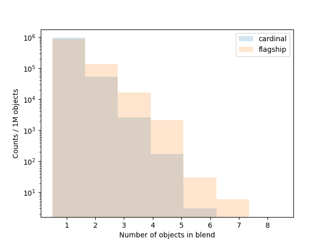
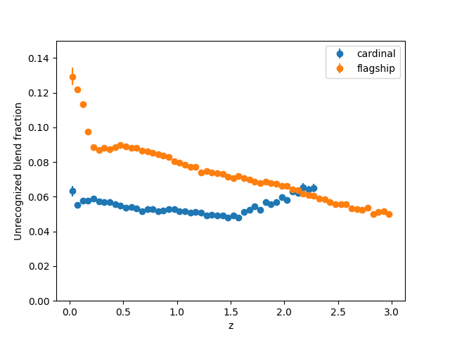
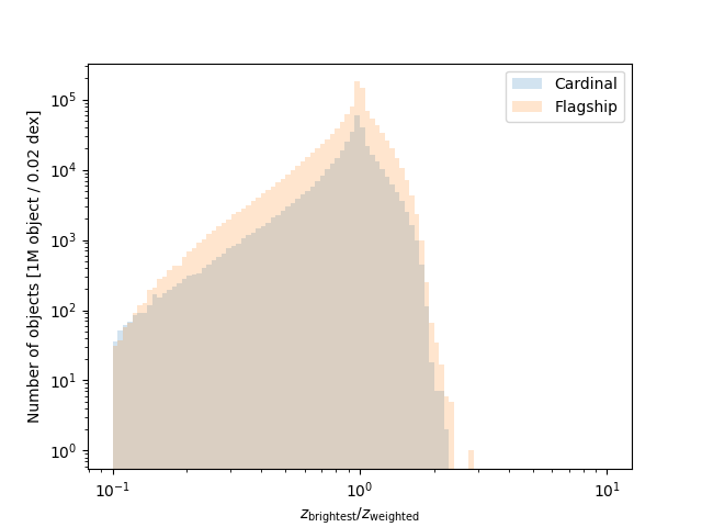
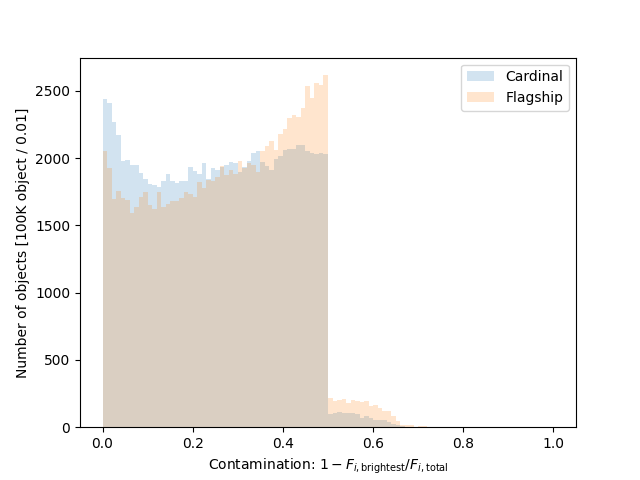
In the files for taskset 4 we emulate the effect of unrecognized blending, i.e., two or more objects being detected as a single object. Our blending algorithm is relatively simple: we apply a “friends-of-friends” matching algorithm with a 1.0 arcsecond linking length replace all groups with a single object with the summed fluxes in each of the bands.
Preparing Training, Test, and Reserved Datasets
All of the data preparation was performed using the rail_projects
and rail_package_config packages for bookkeeping and
reproducibility.
Script |
Command Run |
Purpose |
|---|---|---|
do_00_reduce |
rail-project reduce |
Reduce input truth catalogs |
(mag. cut and drop columns) |
||
do_01_build |
rail-project build |
Build configurations to run |
truth-to-observed pipeline |
||
do_02_t2o |
rail-project run truth-to-observed |
Run truth-to-observed |
pipelines to make degraded catalogs |
||
do_03_merge |
rail-project merge |
Combine spectroscopic selections |
do_04_subselect |
rail-project subsample |
Make train/test files |
from catalogs |
Validation figures
Validation figures for taskset 1
The data preparation for taskset 1 including the following steps:
Starting with either the Cardinal or Flagship simulation truth information.
Rotating the field into an area covered by the LSST survey.
Selecting objects with a true \(i < 25.5\).
Applying photometric smearing. In the Rubin bands this used expected observing conditions and depth maps for 1 and 10 years of observing. In the Roman bands this used the expected depths for the medium tier of the High-Latitude wide area survey.
Drawing training (100k objects) and test (20k objets) data sets from the catalogs, requiring \(i < 23.5\) for both data sets.
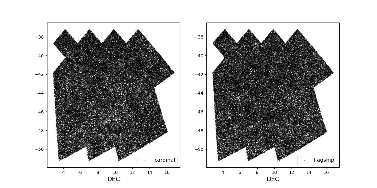
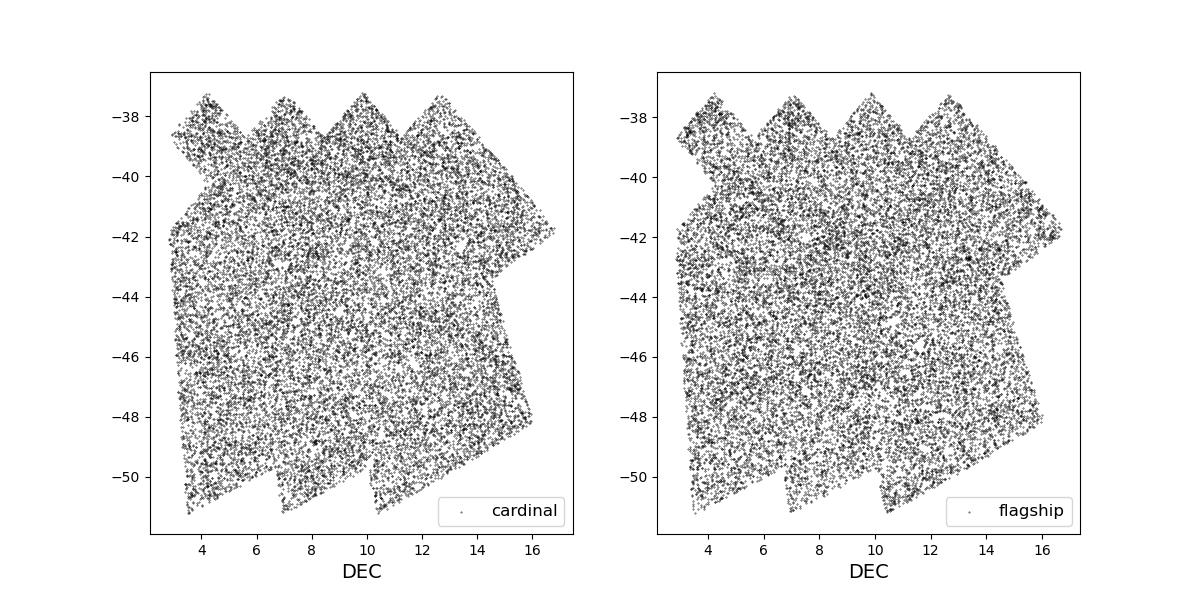
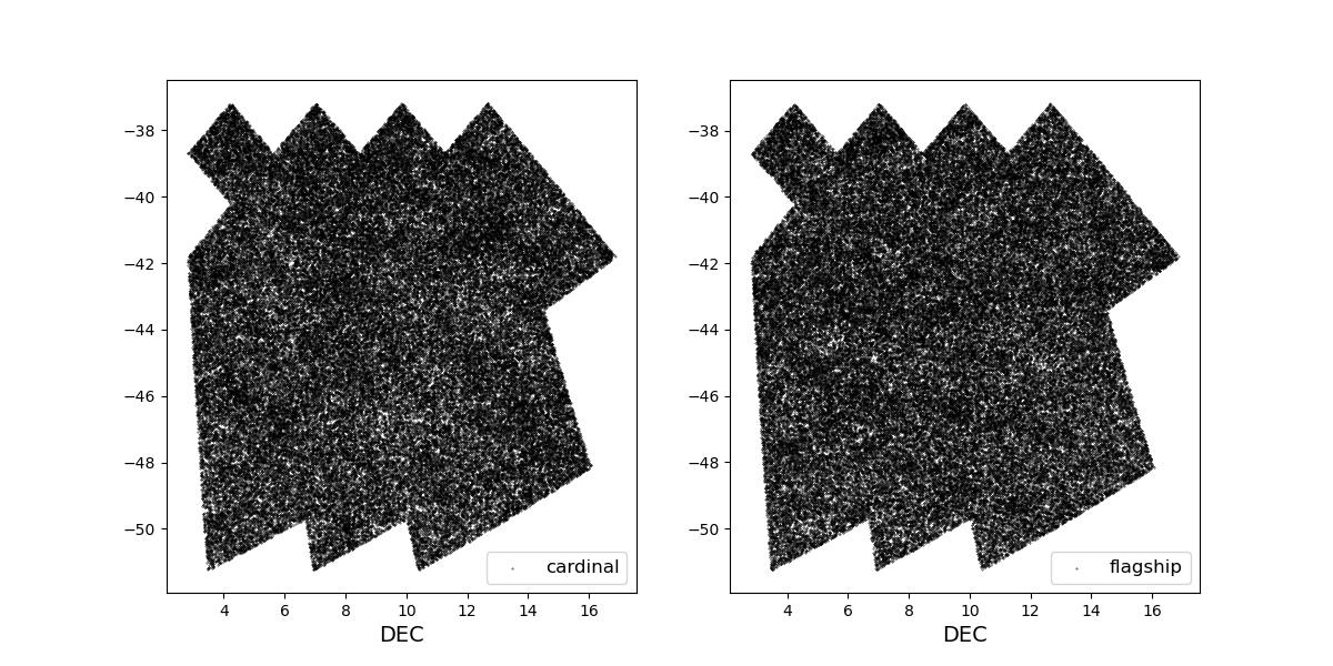
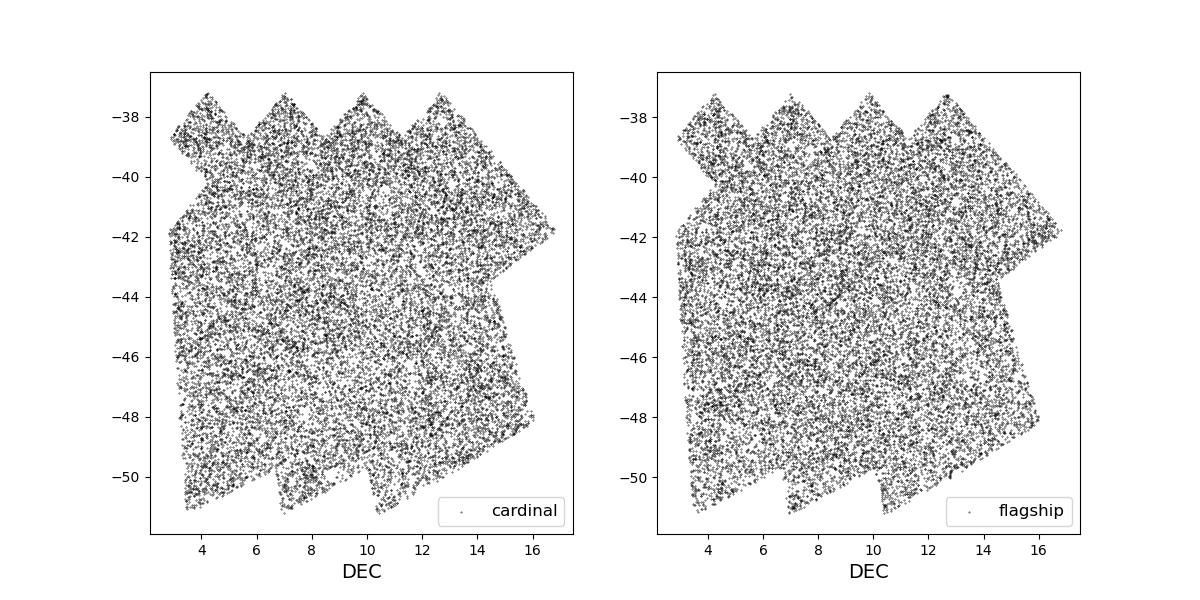
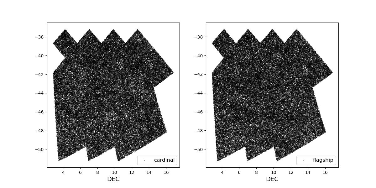
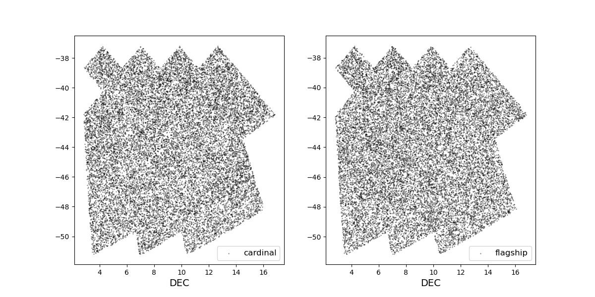
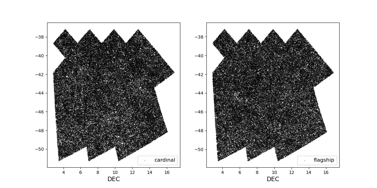
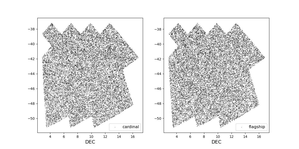
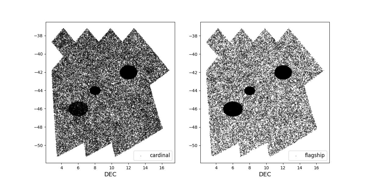
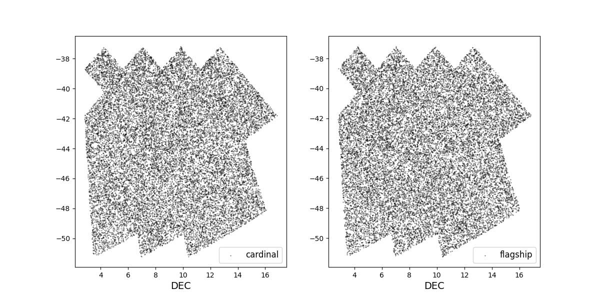
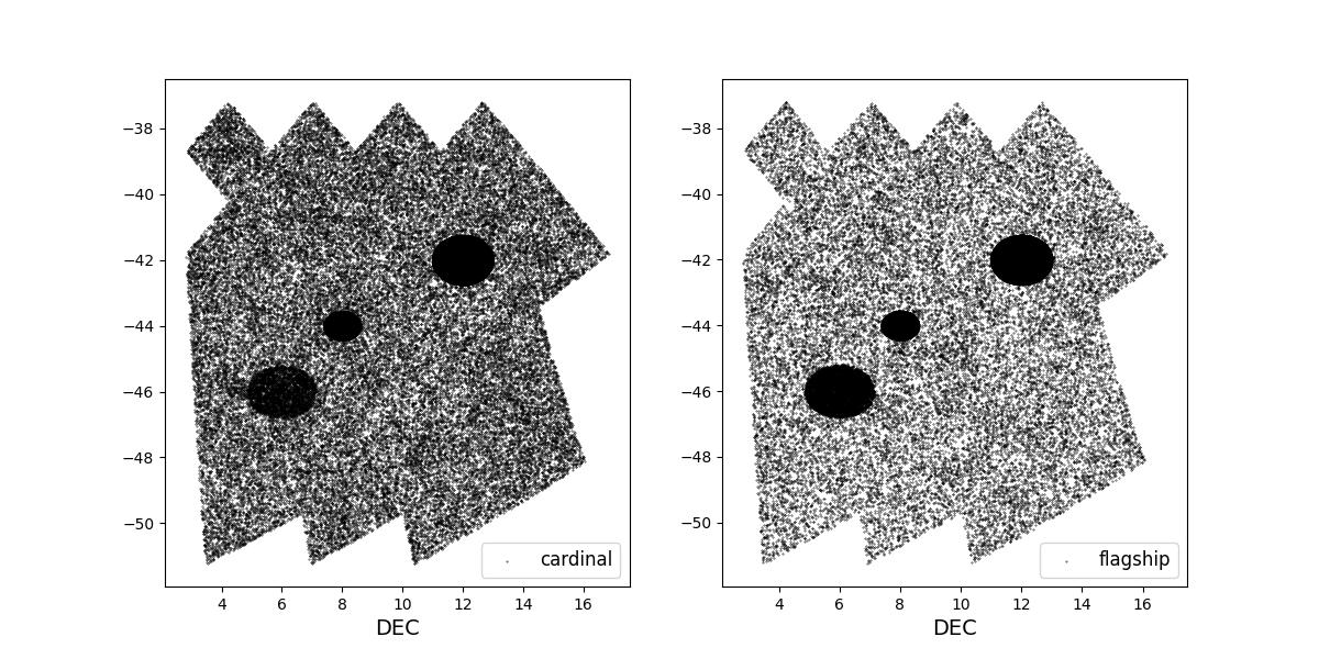
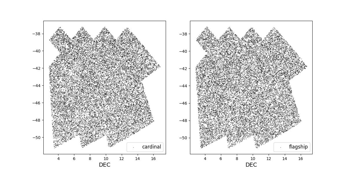
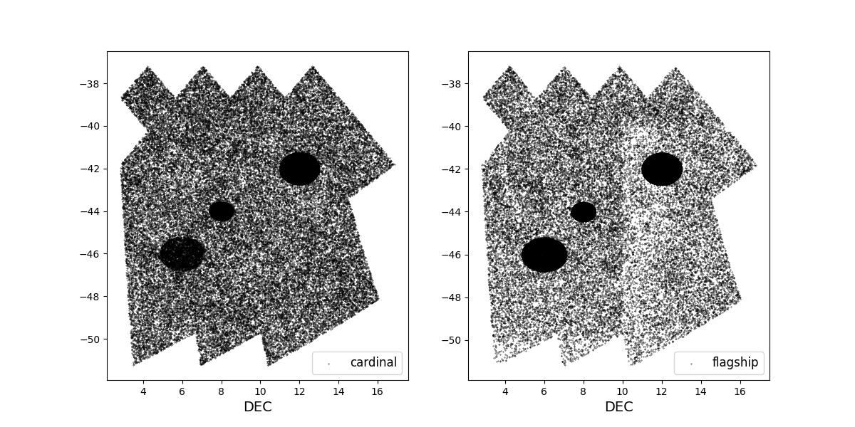
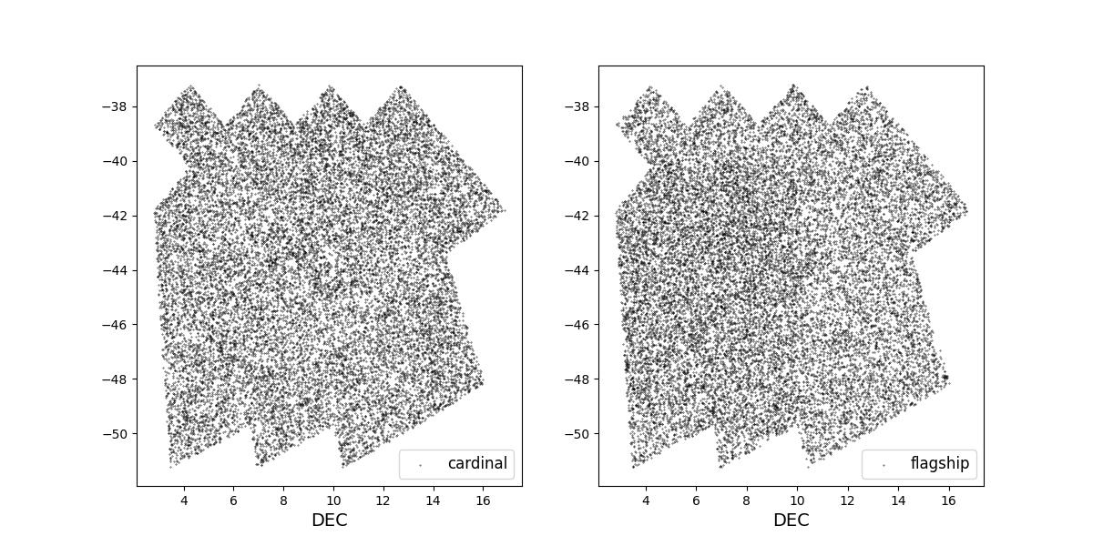
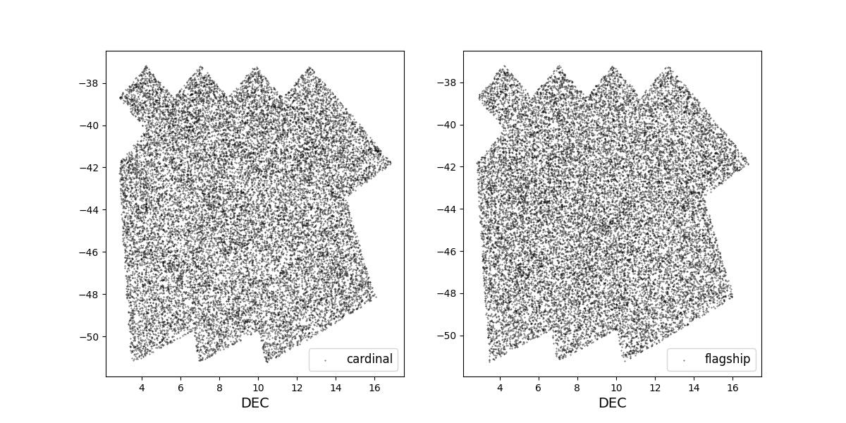
Survey footprints for training (left) and test (right) data. Within each side both 1 cardinal (left) and flagship (right) simulations are shown for both 1 year (top) and 10 year (bottom) data sets.
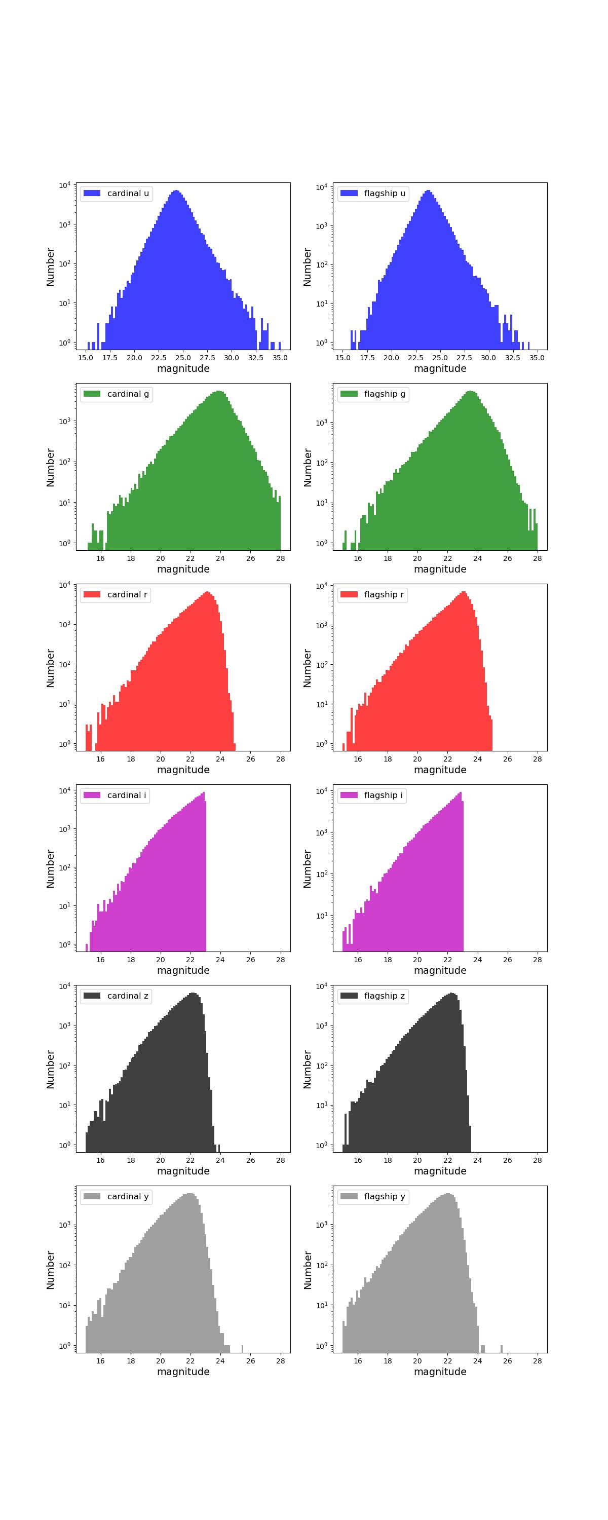
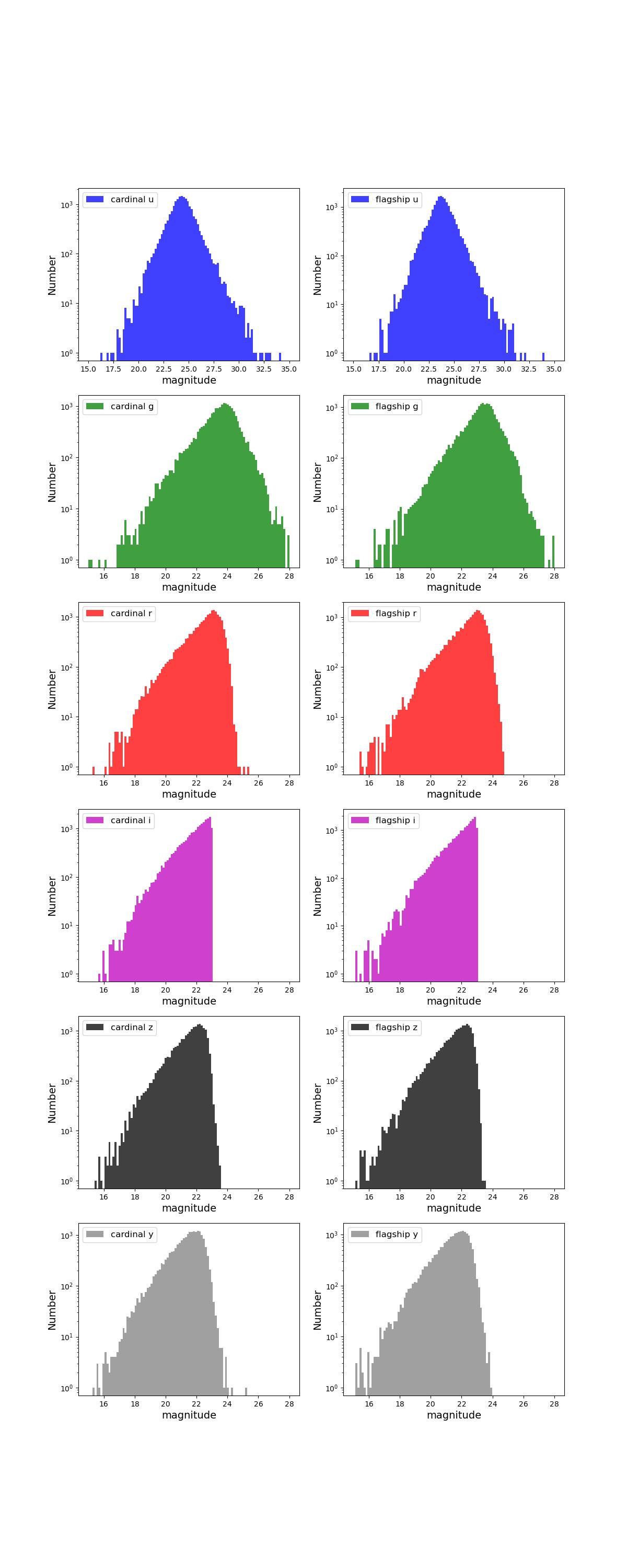
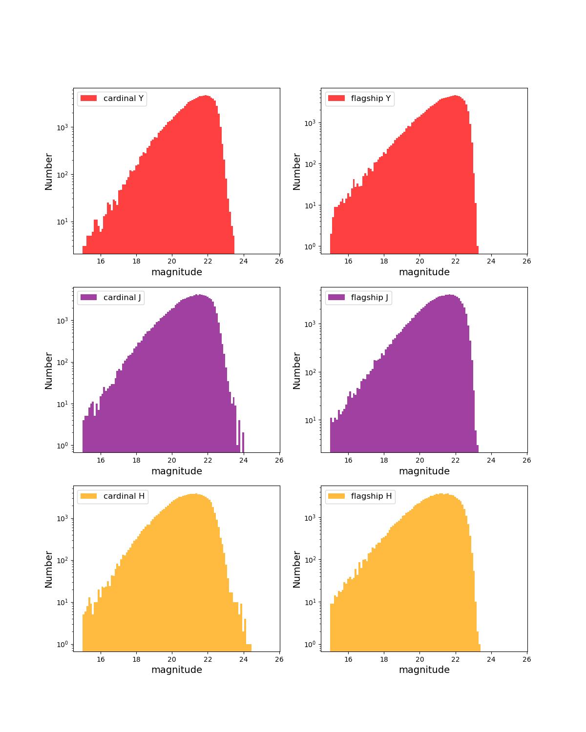
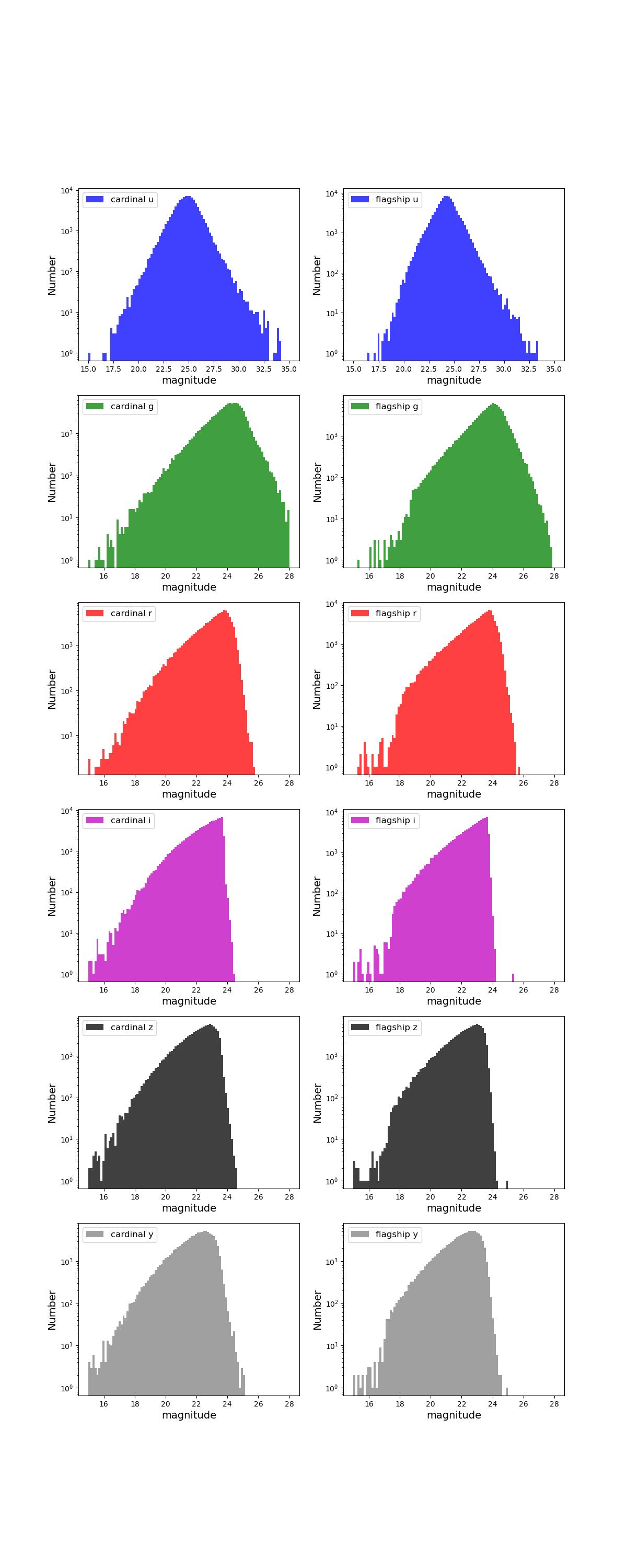
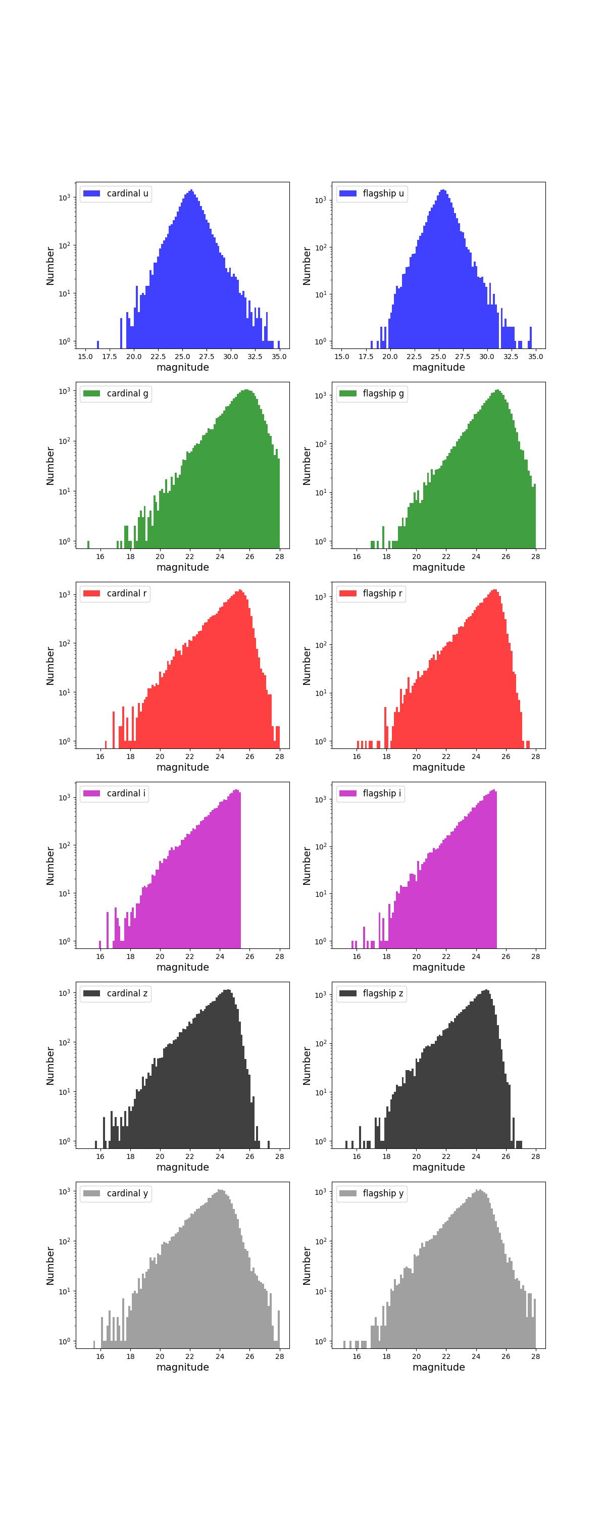
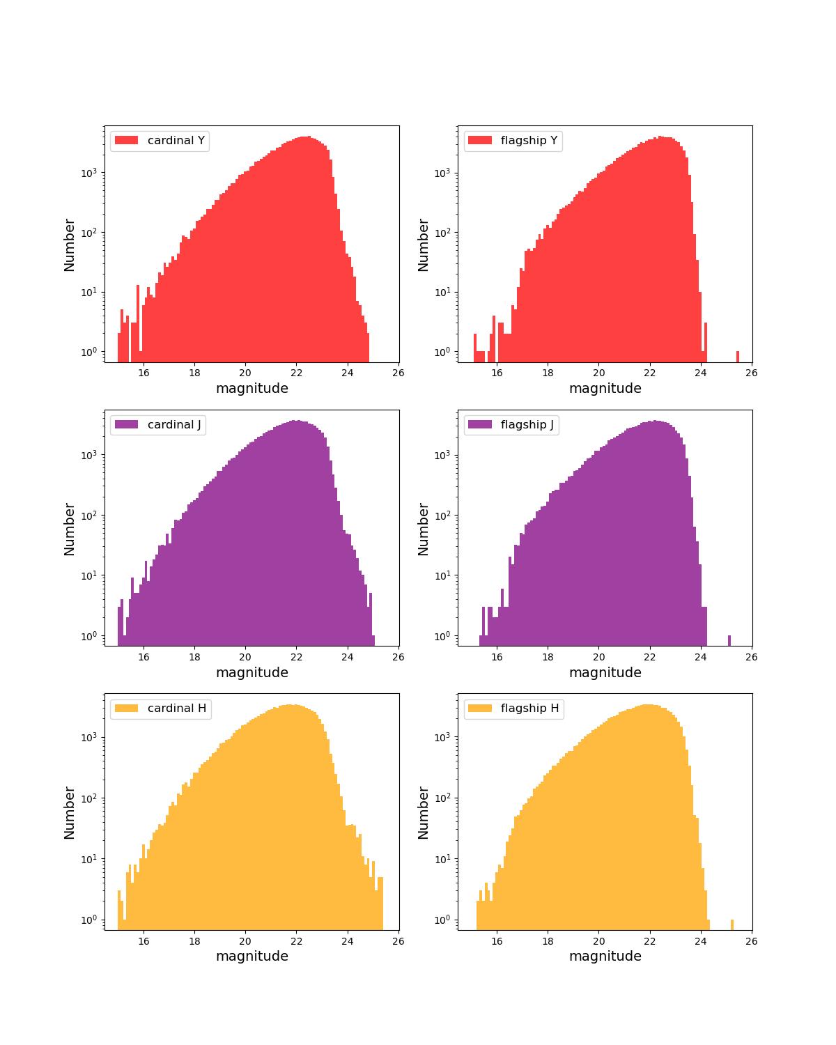
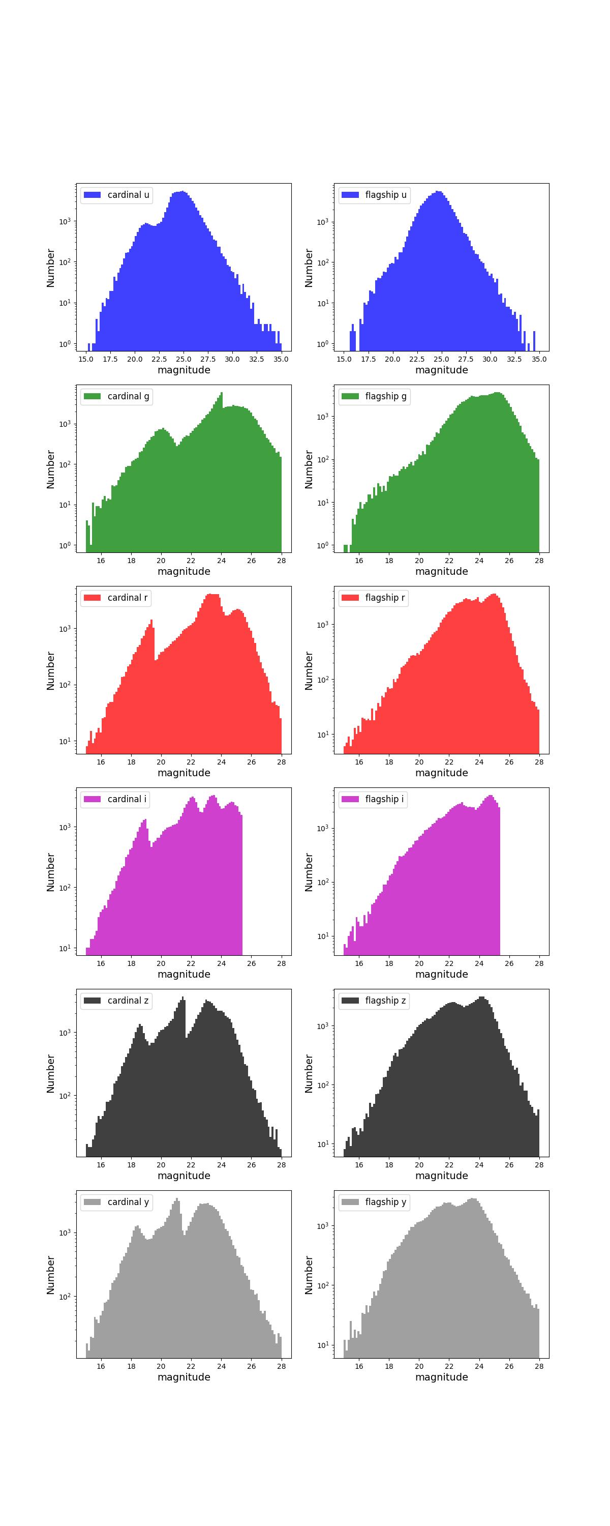
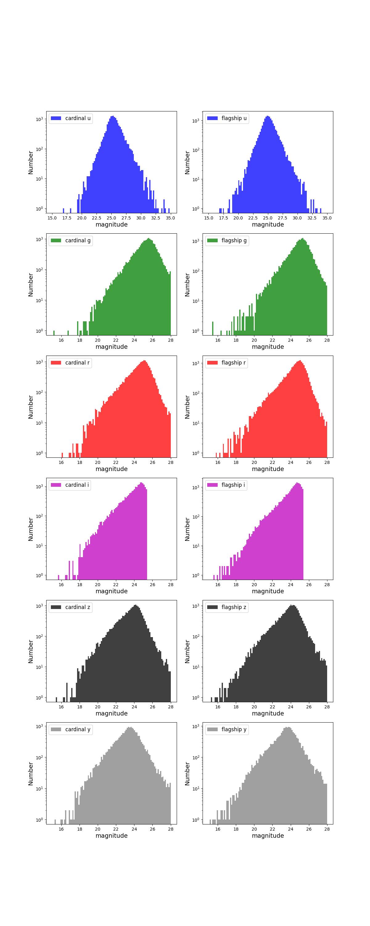
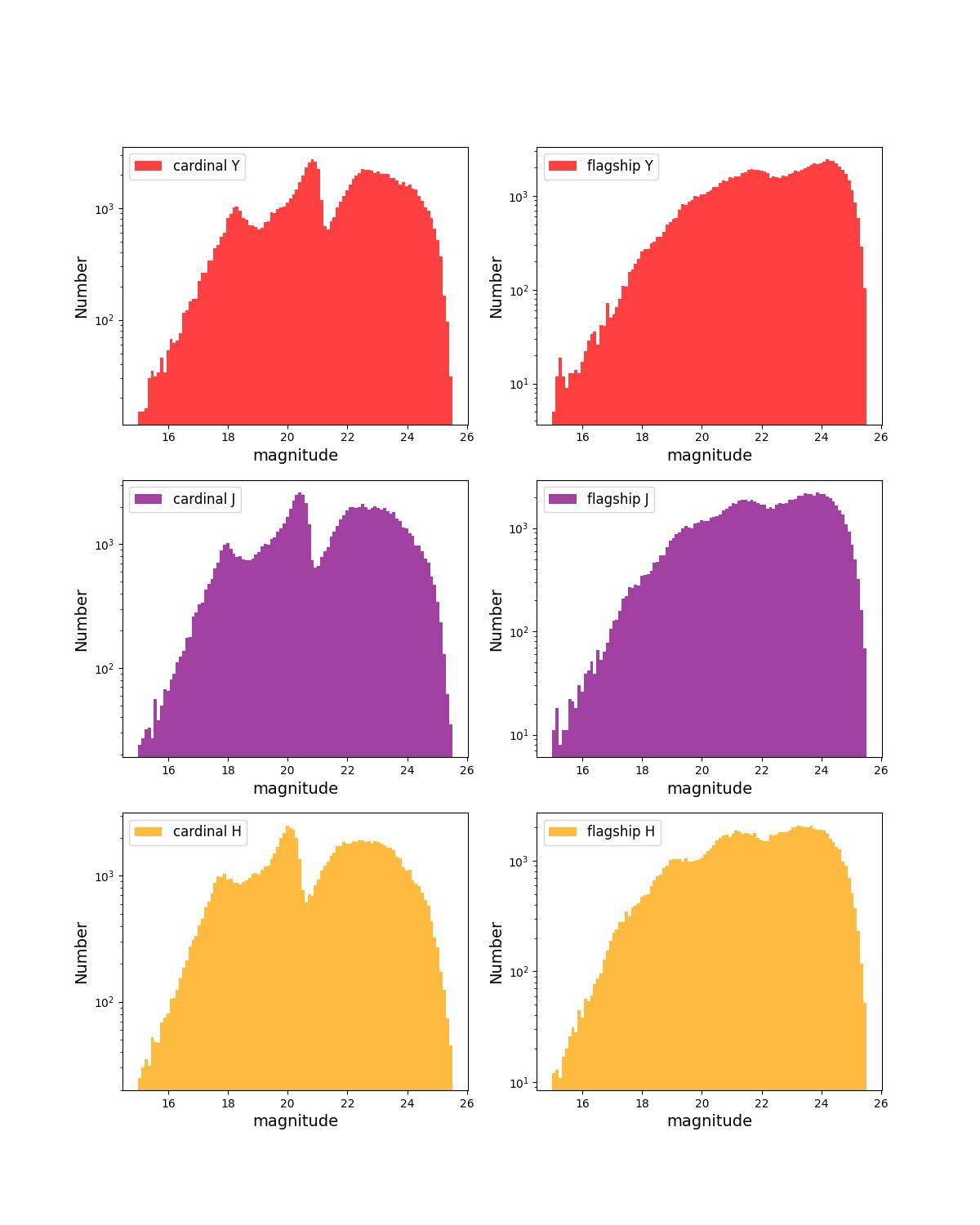
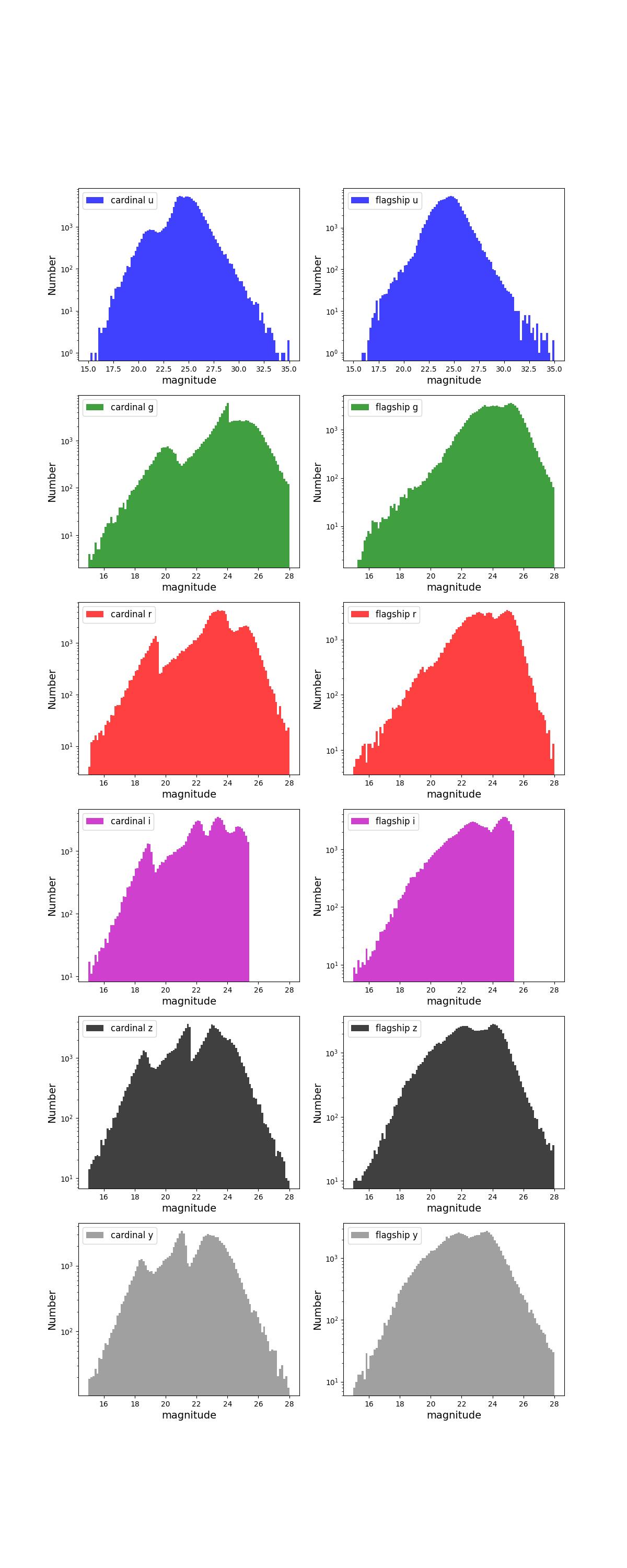
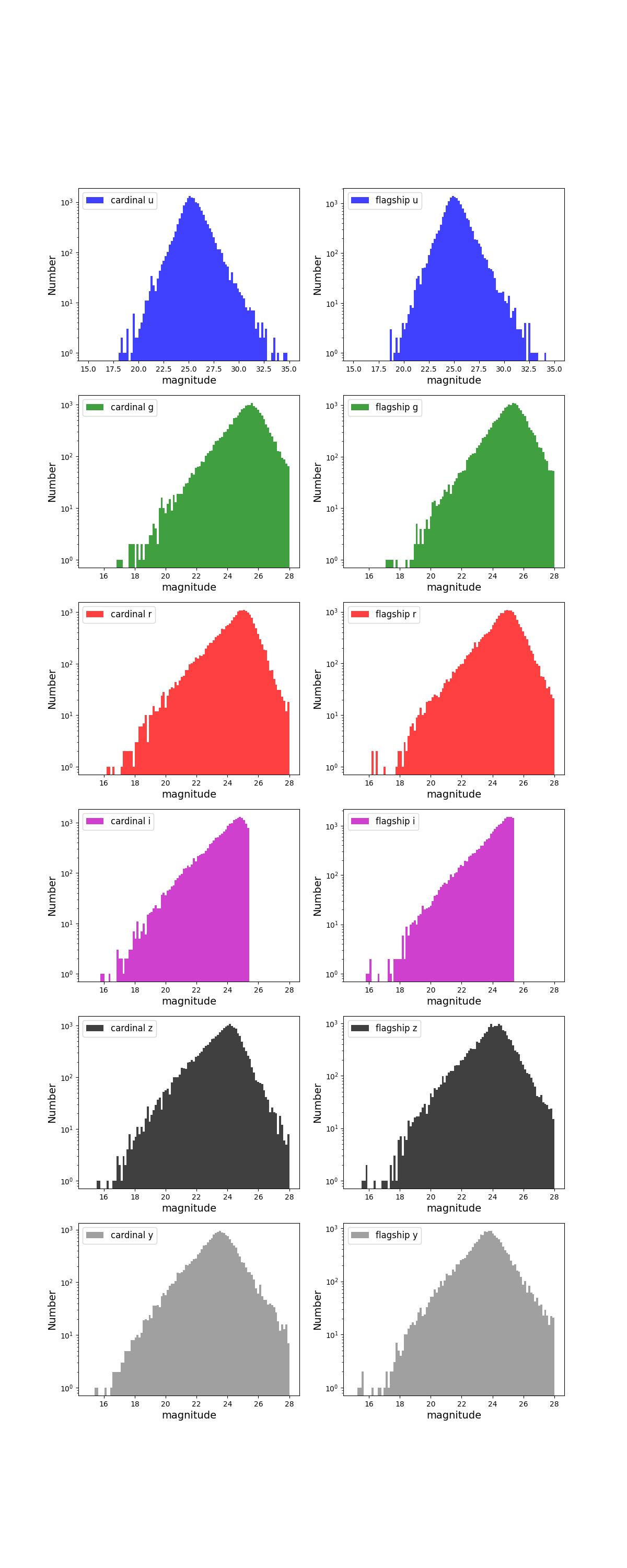
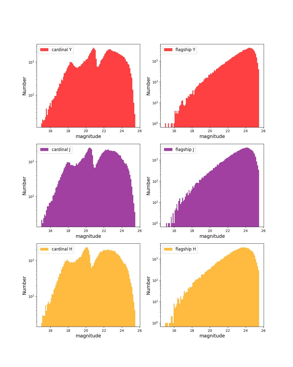
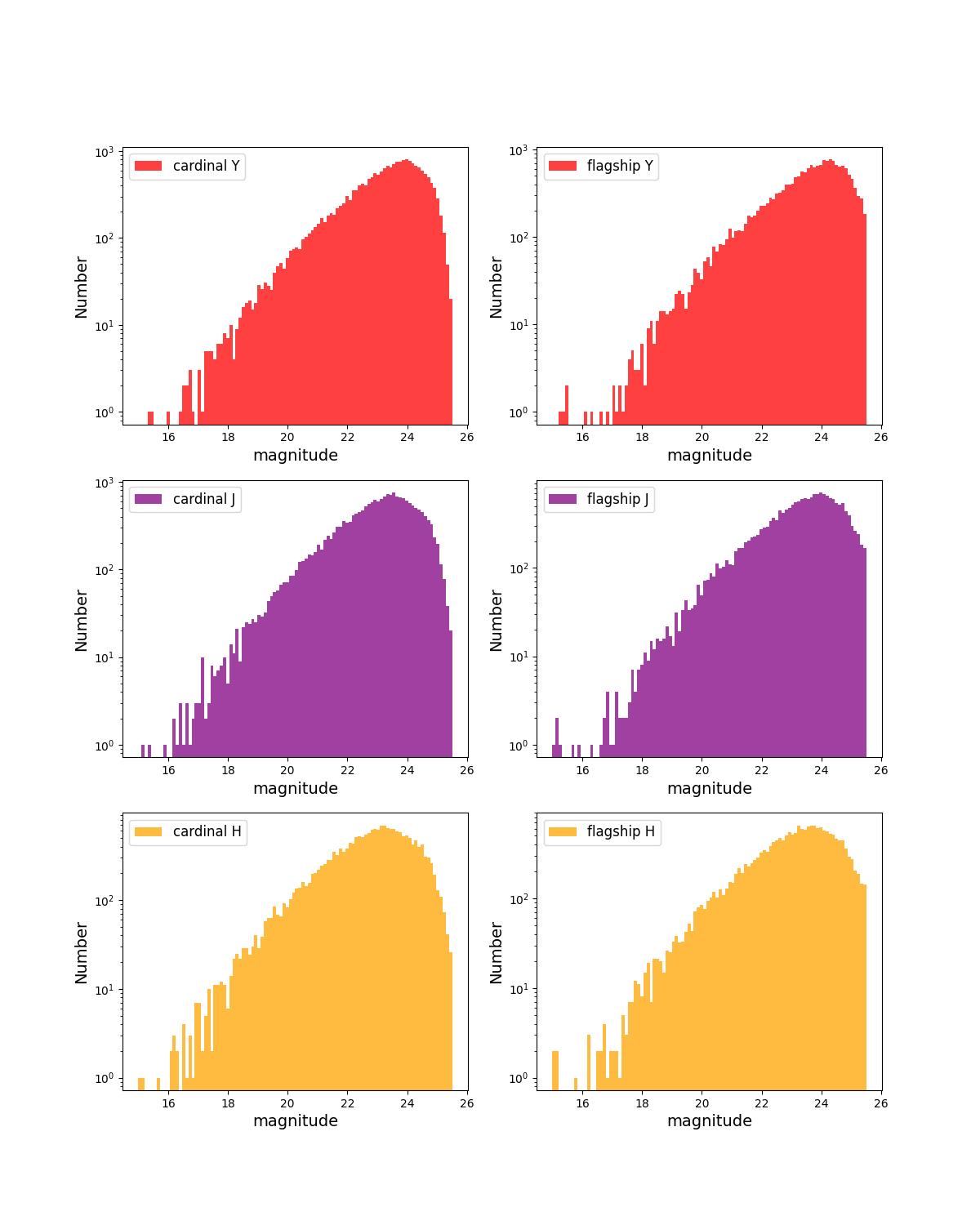
Number counts as a function of magnitude for Rubin (top) and Roman (bottom) bands for 1 year training (left) and test (right) data sets.
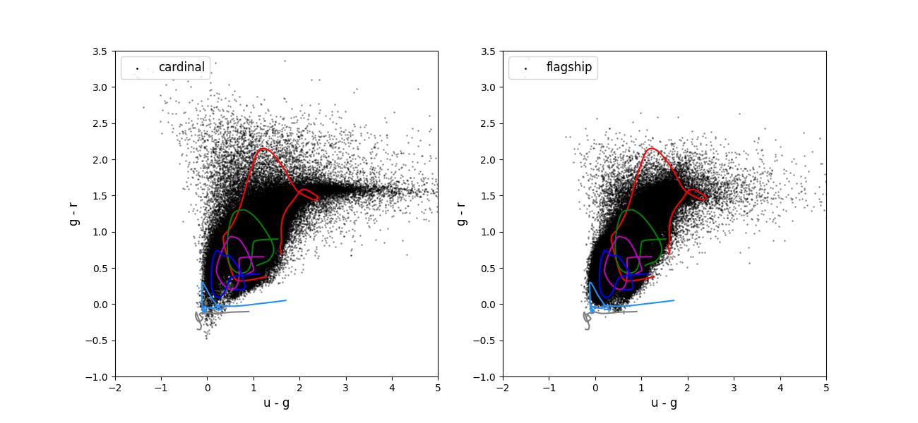
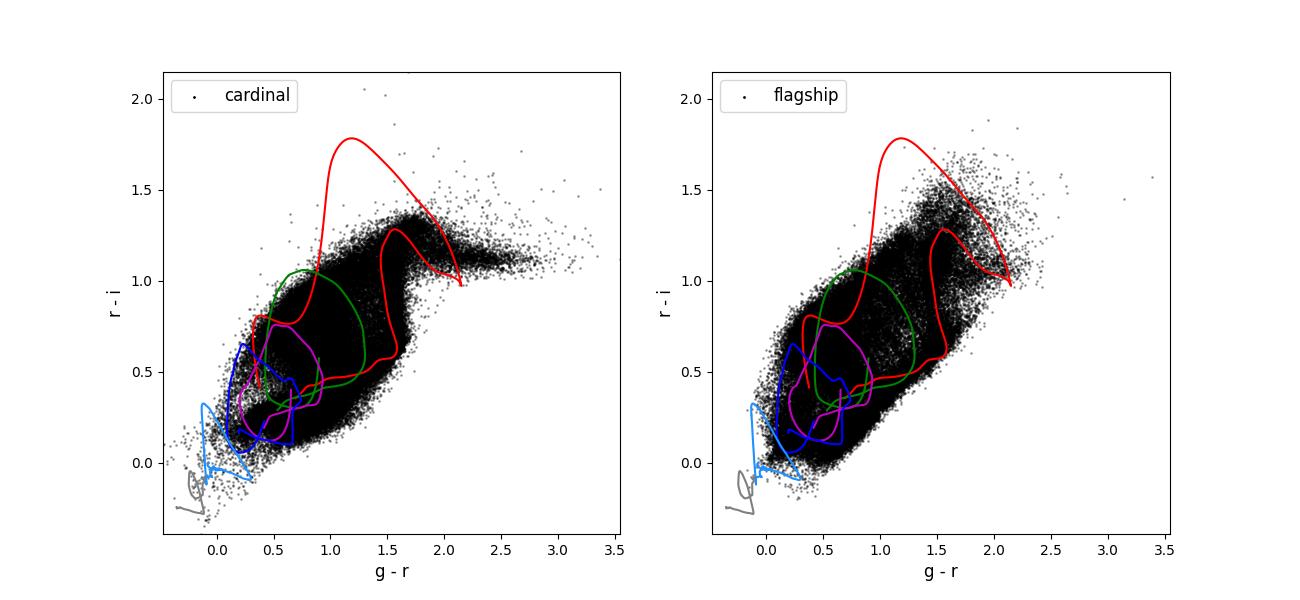
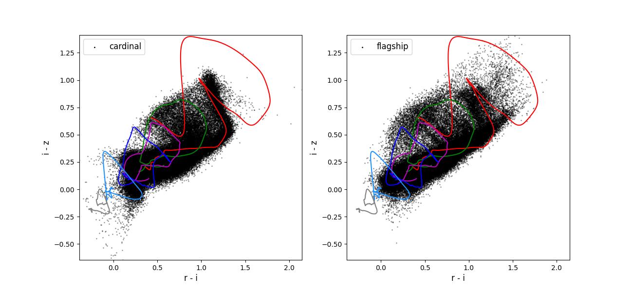
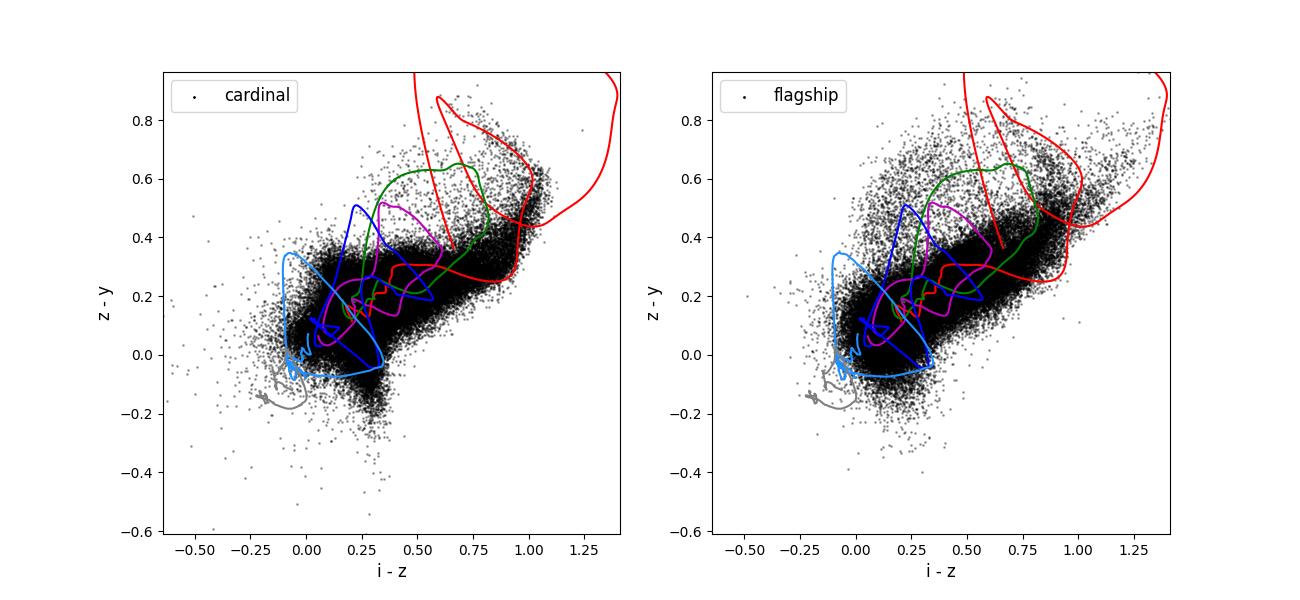
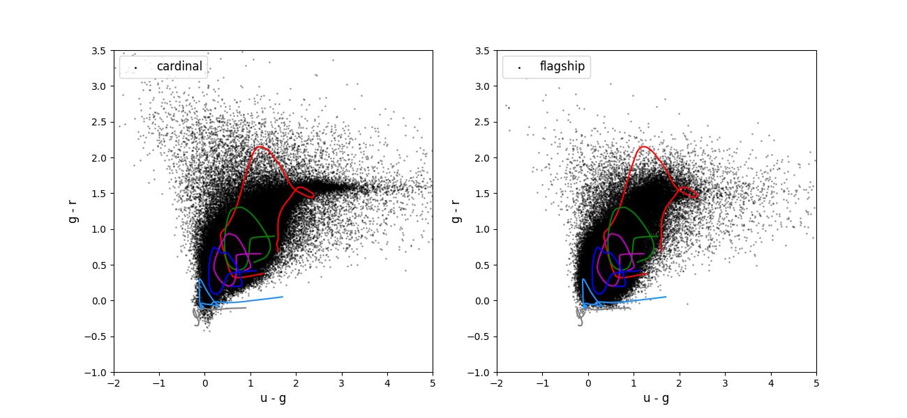
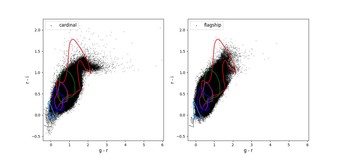
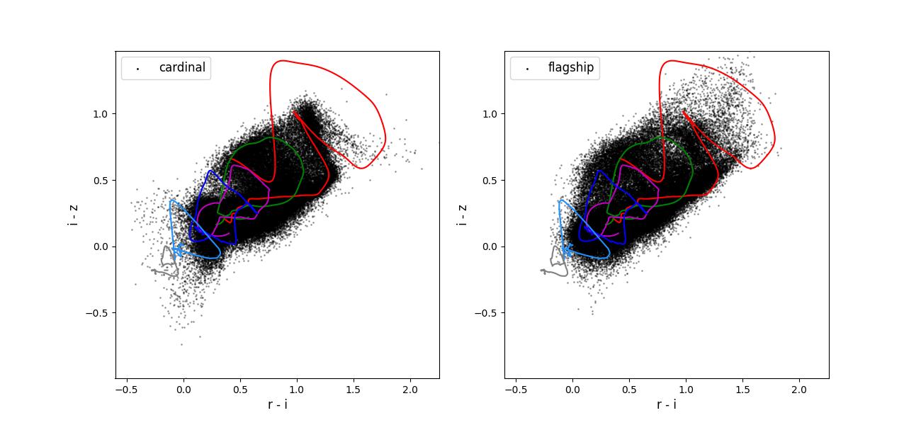
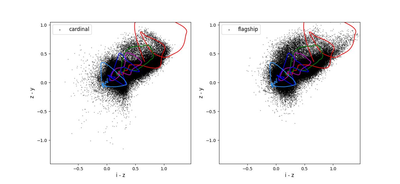
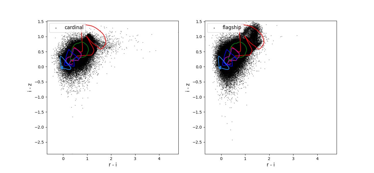
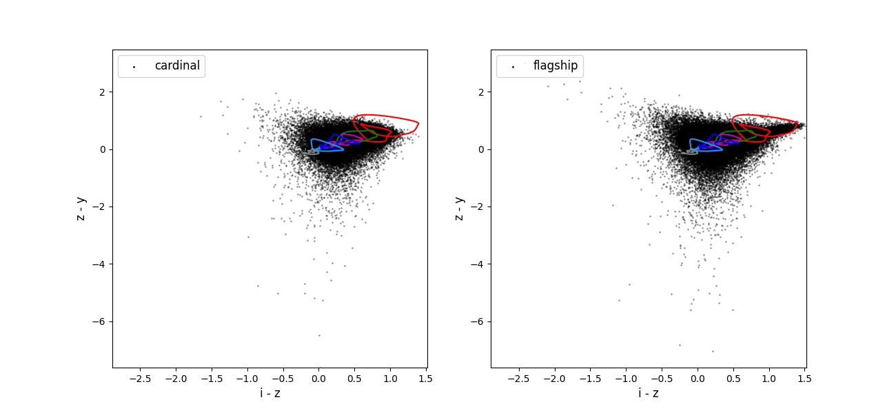
Color-color plots for 10 year training sets pairs of adjacent bands.
Validation figures for taskset 2
The data preparation for taskset 2 including the following steps:
Starting with either the Cardinal or Flagship simulation truth information.
Rotating the field into an area covered by the LSST survey.
Selecting objects with a true \(i < 25.5\).
Applying photometric smearing. In the Rubin bands this used expected observing conditions and depth maps for 1 and 10 years of observing. In the Roman bands this used the expected depths for the medium tier of the High-Latitude wide area survey.
Emulating spectroscopic selections for the reference redshift creation. For this taskset we simply applied the spectroscopic selection functions to the entire field. This will overestimate the number of objects in some of the selections corresponding to surveys that were only performed in small fields.
Drawing a training (100k objects) data set from the objects passing the spectroscopic selections and a test data sets (20k objects) from all the objects with and observed \(i < 25.5\).
Note specifically that the training dataset is not representative of the test data set.
Survey footprints for training (left) and test (right) data. Within each side both 1 cardinal (left) and flagship (right) simulations are shown for both 1 year (top) and 10 year (bottom) data sets.
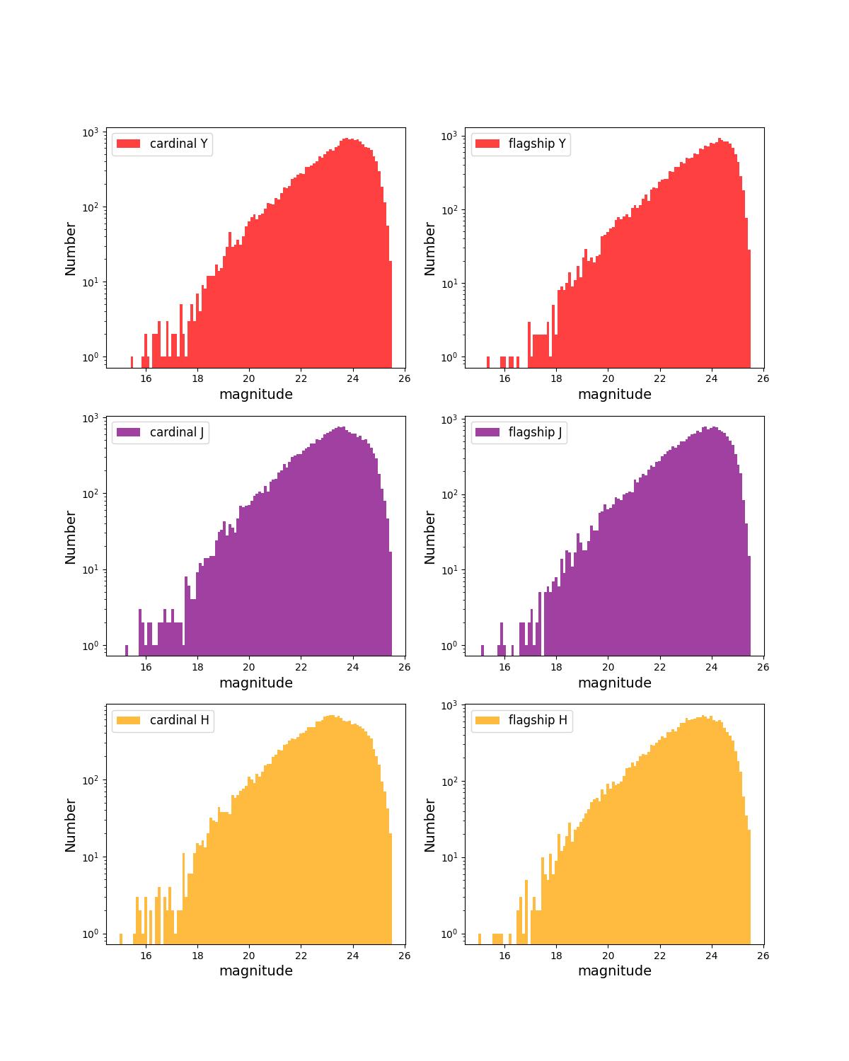
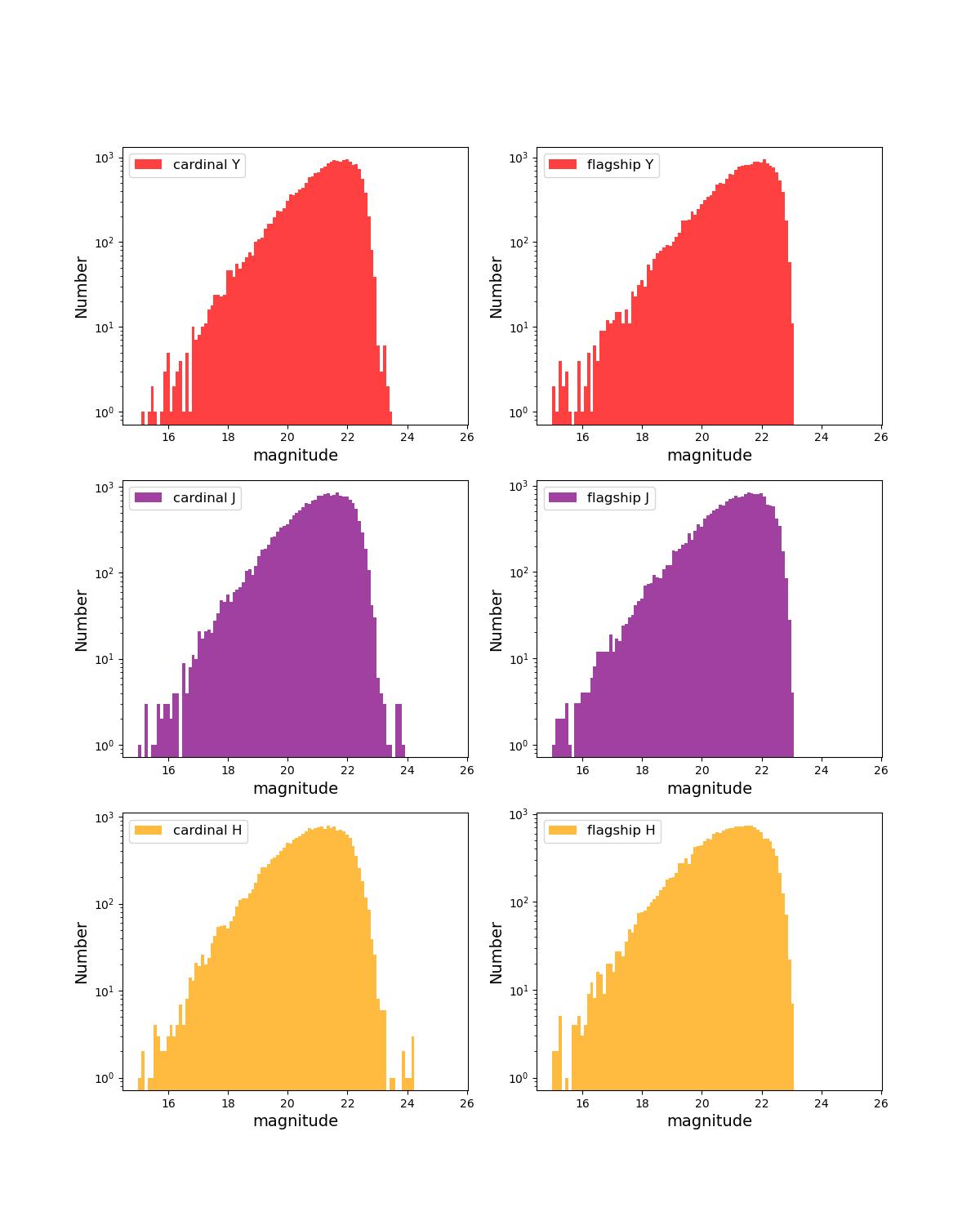
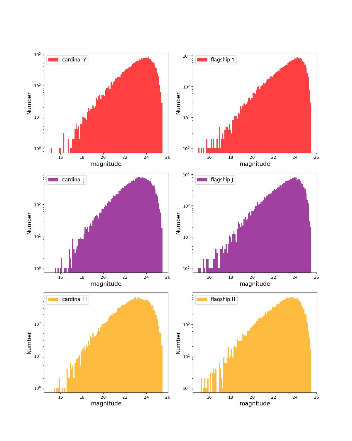
Number counts as a function of magnitude for Rubin (top) and Roman (bottom) bands for 10 year training (left) and test (right) data sets.
Color-color plots for 10 year training sets pairs of adjacent bands.
Validation figures for taskset 3
The data preparation for taskset 3 including the following steps:
Starting with either the Cardinal or Flagship simulation truth information.
Rotating the field into an area covered by the LSST survey.
Selecting objects with a true \(i < 25.5\).
Applying photometric smearing. In the Rubin bands this used expected observing conditions and depth maps for 1 and 10 years of observing. In the Roman bands this used the expected depths for the medium tier of the High-Latitude wide area survey.
Emulating spectroscopic selections for the reference redshift creation. For this taskset we emulate the area of the spectroscopic samples. Specifically, we apply the DESI selections to the whole field, the zCOSMOS and COSMOS2020 selections to the same small area, and the other spectroscopic selections to different small areas. This is intended to give roughly the number of objects we might expect in a joint reference redshift sample.
Drawing a training (100k objects) data set from the objects passing the spectroscopic selections and a test data sets (20k objects) from all the objects with and observed \(i < 25.5\).
Survey footprints for training (left) and test (right) data. Within each side both 1 cardinal (left) and flagship (right) simulations are shown for both 1 year (top) and 10 year (bottom) data sets.
Number counts as a function of magnitude for Rubin (top) and Roman (bottom) bands for 1 year training (left) and test (right) data sets.
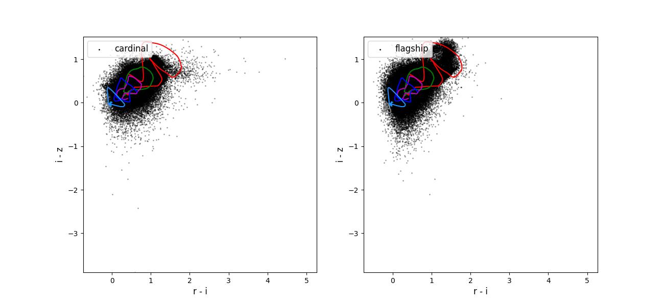
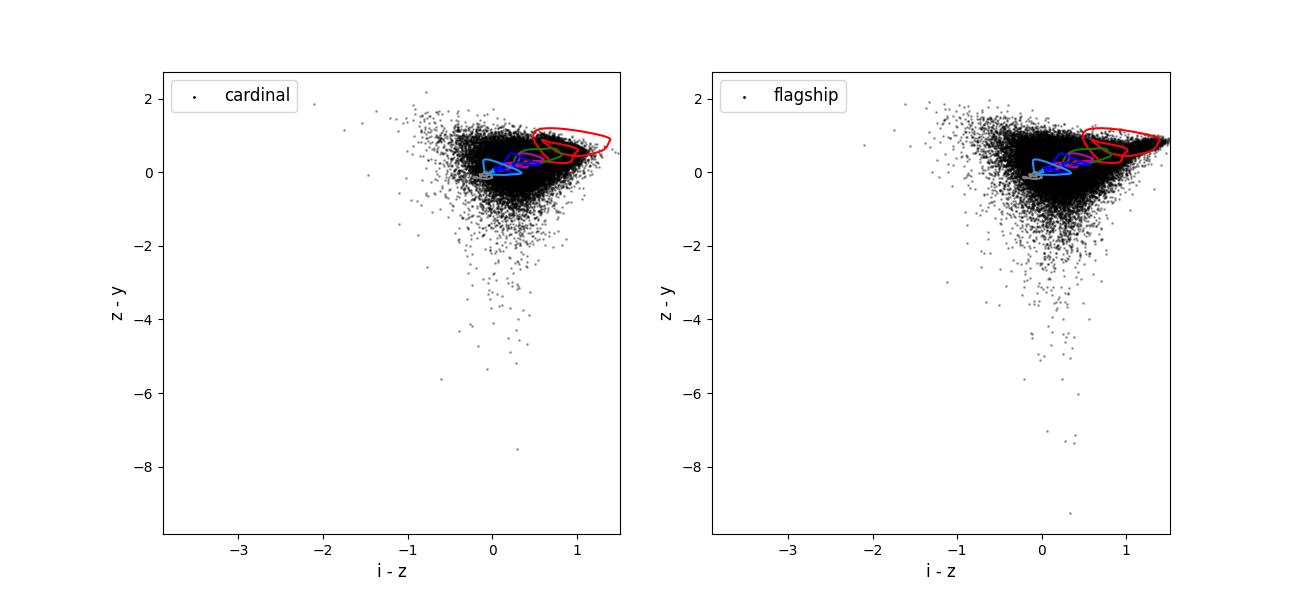
Color-color plots for 10 year training sets pairs of adjacent bands.


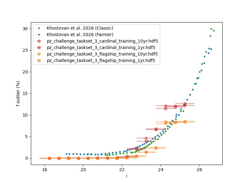
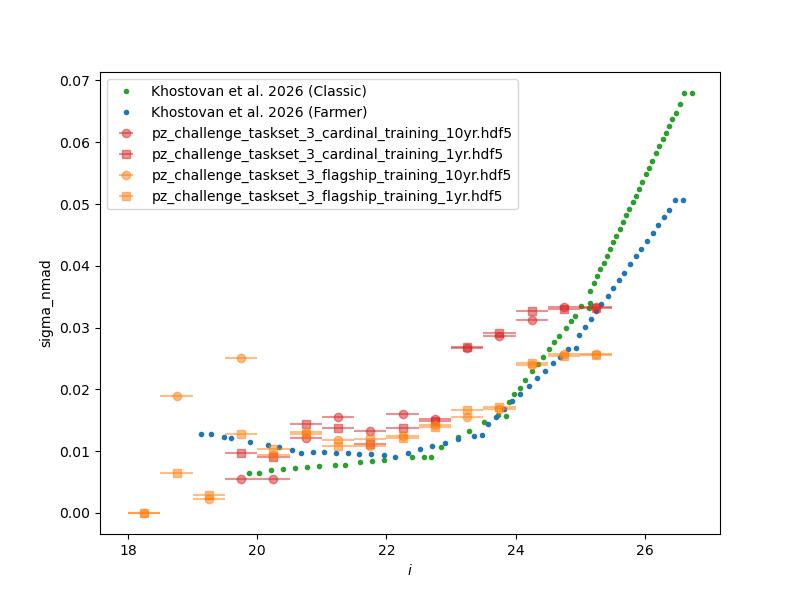
Normalized median absolute deviation (left) and outlier fraction (right) of emulated mock COSMOS2020 photometric redshifts as a function of i-band magnitude for 1 and 10 year training data sets.
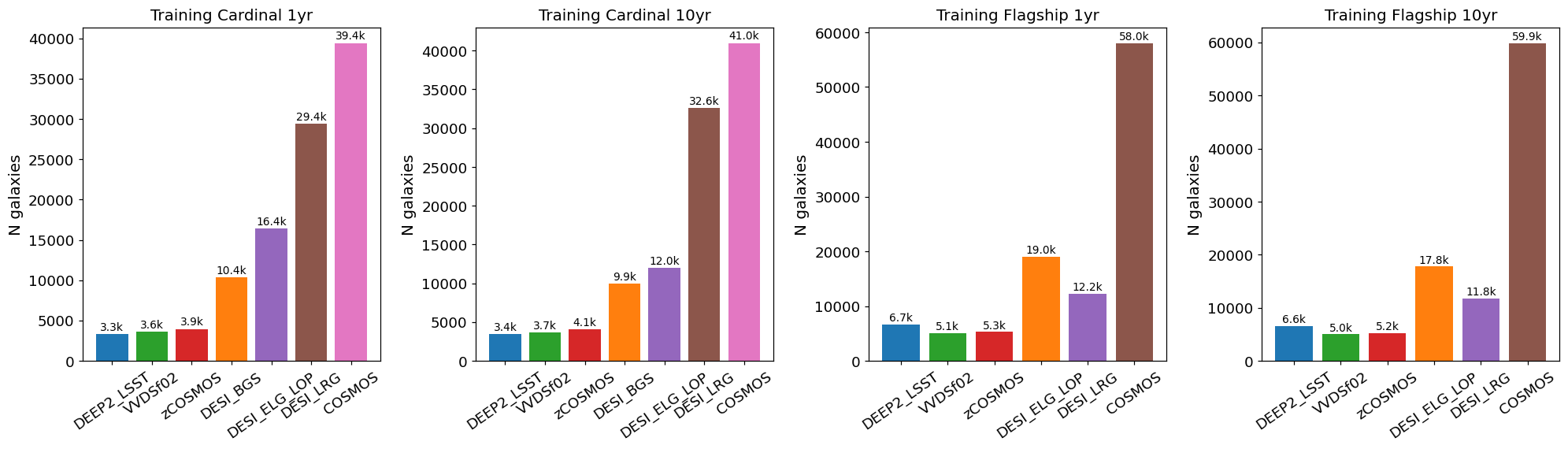
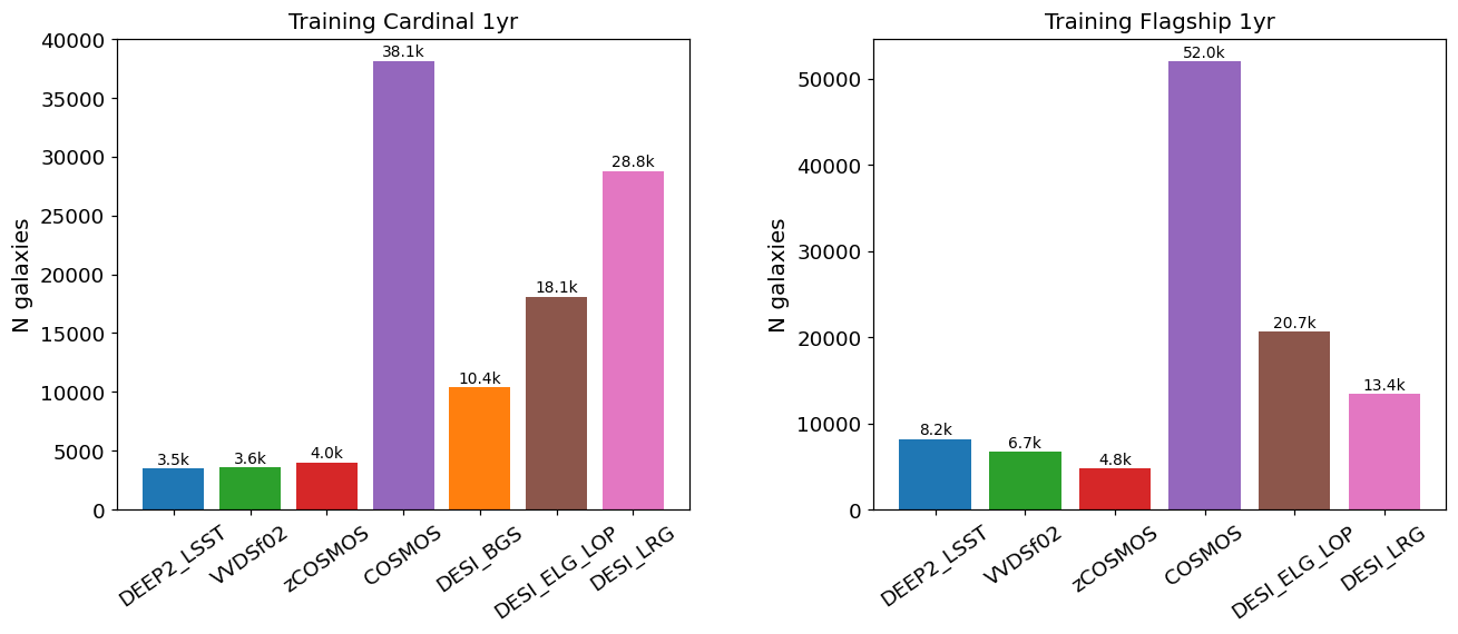
Number of training objects selected by each spectroscopic survey flag (DEEP2, VVDSf02, zCOSMOS, DESI BGS/ELG/LRG, COSMOS) for all four training files (Cardinal and Flagship, 1 and 10 year).
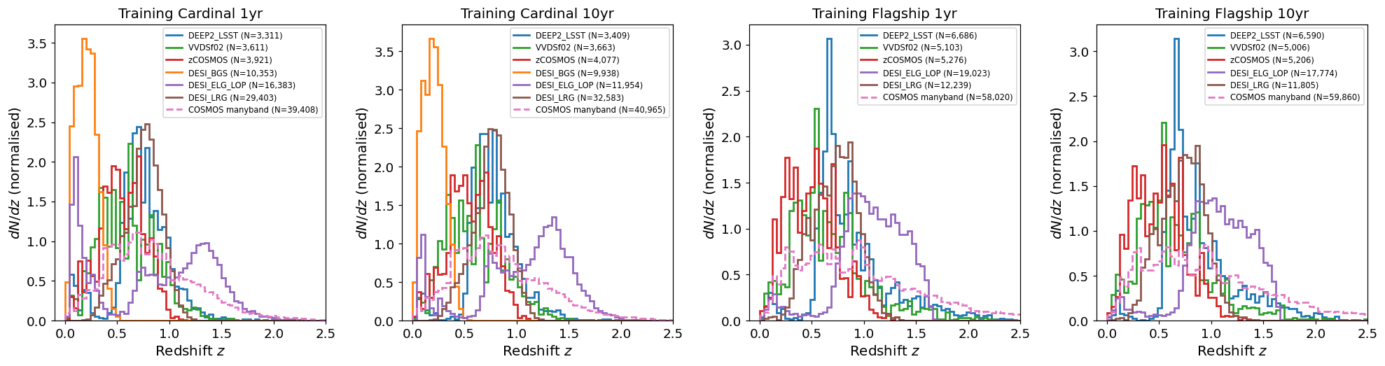
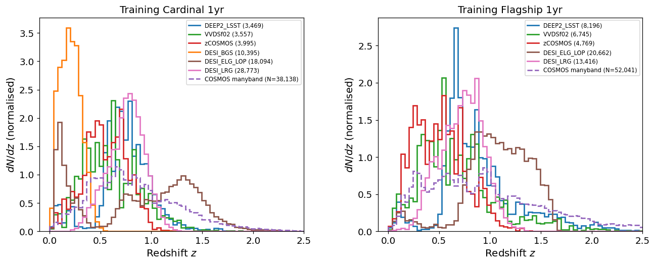
Normalised redshift distributions N(z) of training galaxies split by
spectroscopic survey flag. Each flag selects a distinct redshift range
reflecting the target selection of the underlying survey. The dashed
pink curve shows N(z) derived from the many-band photometric redshift
(redshift_manyband) for COSMOS-selected objects, whose true
spectroscopic redshifts are not available.
Validation figures for taskset 4
The data preparation for taskset 4 including the following steps:
Starting with either the Cardinal or Flagship simulation truth information.
Rotating the field into an area covered by the LSST survey.
Selecting objects with a true \(i < 27.0\).
Blending objects within the Rubin PSF into single objects by combining their fluxes. After the blending we only retain objects with \(i < 25.5\). For blended objects, we assign the blend the true redshift of the brightest object in the blend.
Applying photometric smearing. In the Rubin bands this used expected observing conditions and depth maps for 1 and 10 years of observing. In the Roman bands this used the expected depths for the medium tier of the High-Latitude wide area survey.
Emulating spectroscopic selections for the reference redshift creation. For this taskset we emulate the area of the spectroscopic samples. Specifically, we apply the DESI selections to the whole field, the zCOSMOS and COSMOS2020 selections to the same small area, and the other spectroscopic selections to different small areas. This is intended to give roughly the number of objects we might expect in a joint reference redshift sample.
Drawing a training (100k objects) data set from the objects passing the spectroscopic selections and a test data sets (20k objects) from all the objects with and observed \(i < 25.5\).

Survey footprints for training (left) and test (right) data. Within each side both 1 cardinal (left) and flagship (right) simulations are shown for both 1 year (top) and 10 year (bottom) data sets.
Number counts as a function of magnitude for Rubin (top) and Roman (bottom) bands for 1 year training (left) and test (right) data sets.

Color-color plots for 10 year training sets pairs of adjacent bands.
Number of training objects selected by each spectroscopic survey flag (DEEP2, VVDSf02, zCOSMOS, COSMOS, DESI BGS/ELG/LRG) for Cardinal and Flagship 1-year training files. Taskset 4 training is 1-year only; no 10-year training data is provided.
Normalised redshift distributions N(z) of training galaxies split by
spectroscopic survey flag. The dashed purple curve shows N(z) derived
from the many-band photometric redshift (redshift_manyband) for
COSMOS-selected objects, whose true spectroscopic redshifts are not
available.